Intra-system Interference Analysis

Overview

Intra-system interference is calculated in the network display. The calculation is organized in groups. Only visible layers will be used in the calculation. All sites and links which are not on a visible layer will be ignored. The calculations use antenna and radio data files. These contain the parameters required for an interference calculation and are described in detail in this section. The minimum conditions to calculate intra-system interference are listed below:

A Pathloss data file (pl4, pl5, pl6 or plz) must be associated with each link to be used in the calculation.
An antenna data file must be specified for each antenna in the Pathloss data file.
The Transmission Analysis must be complete to the level of a receive signal calculation.
Transmit and receive frequency assignments must be specified for the Pathloss data files used in the calculation.

A radio data file is optional; however, only the interfering level can be calculated without this file. This file is required to calculate filter improvement and threshold degradation.

Note that there is no provision to calculate the interference from a transmitter into a receiver located at the same site.

On completion of an interference calculation, the user is prompted to save the calculation results. The default file name is the GR5 file name with the extension IFR. The file can be reloaded provided that the current GR5 file was used to create the interference file or the network display is blank.

Interference Calculation Procedure

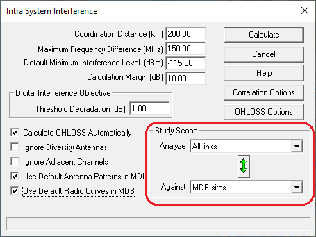
Select the Interference - Calculate interference menu item on the network display menu bar. The Intra-System Interference dialog box sets the options for the calculation.

Study Scope

Interference is calculated between two sets of links. One set of links can act as the interfering transmitters and the other as the victim receivers or both sets can act as interfering transmitters. These sets of links can be a selection, a named group of links, all links or the master database.

Select the two sets of sites and click on the green arrow to change between a single direction and bidirectional analysis. Note that if the two sets are the same, then the calculation is inherently bidirectional and the specified direction has no effect.

When analyzing one set of links against second set of links, it is expected, that the user will define two independent sets without any overlapping links. In the case of overlapping links, the analysis in the overlap area will produce duplicate interference cases. These duplicates are removed from the results; however, as a cautionary measure, the user is advised to examine the cross reference report to verify that duplicates are not present.

When an interference analysis between the network display and the master database is carried out, duplicate interference cases can also occur. In this case, the test for duplicate interference cases can be ambiguous and the user is responsible to delete any duplicates.

Digital Interference Objective

The objective is specified in terms of the allowable receiver threshold degradation. For frequency coordination with other operators, the usual value is 1 dB; however, for intra-system interference, the final criteria is determined by the increased outage times resulting from the actual threshold degradation.

Note that the allowable threshold degradation determines the composite interfering level. A calculation margin described below is subtracted from this composite interfering level to established a reporting threshold level. The following example illustrates this procedure.

Threshold Degradation	1 dB - user specified
Receiver Noise Floor	-107 dBm - calculated from RX threshold data
Interfering Level	-113 dBm - calculated from receiver noise floor and threshold degradation
Calculation Margin	10 dB - user specified
Reporting Threshold	-123 dBm - all interfering signals below this level will be ignored

Sometimes an analysis shows that there are no interference cases and the user would like to examine all interference calculations. This can be accomplished by lowering the reporting threshold using a threshold degradation of 0.01 dB and a calculation margin of 200 dB. In the above example, these values would result in a reporting threshold of -333.5 dBm which will show all cases in any practical system

Default Minimum Interference Level

In the above reporting threshold example, the interfering level required to meet the threshold degradation objective was calculated from the receiver noise floor. In the event that the receiver noise floor is not available, the default minimum interference level will be used as the interfering level required to meet the threshold degradation objective. The reporting threshold level will then be given by the default minimum interference level minus the calculation margin.

Calculation Margin

The calculation margin sets a tolerance on the reporting of interference cases. If the interference level objective for the receiver under test is -104 dBm and the calculation margin is set to 10 dB, then all interference cases greater than -114 dBm (-104 - 10) will be reported.

The threshold degradation objective will be converted to an interference level objective for each receiver in the calculation.

Coordination Distance

Interference is not calculated if the interfering path length is greater than the specified coordination distance.

Maximum Frequency Separation

Interference is not calculated if the difference between the interfering transmitter and victim receiver frequencies is greater than the specified maximum value.

Note that if a radio data file is not available, a co-channel interference analysis can be carried out by setting the maximum frequency separation to some value less than the TX to RX frequency spacing.

Ignore Diversity Antennas

This option ignores all receive frequencies associated with a space diversity receive only antenna. In the initial frequency analysis, this option will reduce the number of cases by 50%. If the main and diversity antenna gains are different, then the final analysis should consider the diversity antennas.

Ignore Adjacent Channels

This option applies to 1 for N systems. Once the threshold degradation of the adjacent channels has been established, use this option to limit the number of interference cases.

Calculate OHLOSS Automatically

This option will automatically calculate the over the horizon loss (OHLOSS) on all interfering paths which do not have a direct link to the affected receiver. Click the OHLOSS option button to set the specific options for the OHLOSS calculation.

OHLOSS calculations can be a contentious item when resolving interference case between different organizations It is important to note that if an OHLOSS calculation results in a interfering level below the reporting threshold, the interference case will not appear in any report. If the OHLOSS calculations are carried out in the case detail report screen after the main calculation is complete, the OHLOSS cases will remain in the analysis.

OHLOSS Options

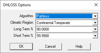Click the OHLOSS options button in the Intra system interference dialog. These options will be used in all OHLOSS calculations in the present analysis. Refer to the help in the Diffraction module for complete details on the OHLOSS calculation procedure.

An OHLOSS calculation takes time variability into account. Current practice is to compute a long term and a short term time variability. The long term is normally set to 80%. Threshold degradation objectives refer to this long term objective. In the short term, the allowable threshold degradation can be significantly higher.

If required set the diffraction algorithm, the climatic region and the short and long term time percentages.

More information on OHLOSS (Over the Horizon Loss)

Correlation Options

When an interfering path is the same as the desired path, the interference case is defined as correlated.

In the diagram on the right, the Site 1 receiver from Site 2 is being interfered with the Site 2 transmitter towards Site 3. The main path is from Site 2 to Site 1 and the interfering path is also from Site 2 to Site 1. Therefore this is a correlated interference case

In this case it is expected that fading on the interfering main paths will occur at the same time. In the case of multipath fading, the actual fade depths on the two paths will depend on the type of correlation. If the interfering transmitter antenna heights are the same as the main transmitter heights, then the two paths are completely correlated. In this case it is common practice to ignore the case, particularly if automatic transmit power control is employed. The main path will increase power in response to the fade; however the interfering transmitter may not change.

A partially correlated situation exists when the interfering transmitter antenna height is different than the main transmitter antenna height. In this case, an additional loss in the order of 5 to 10 dB is added to the interfering signal

Although the same correlation options are used for both multipath and rain, the definition of correlation is actually whether the interfering and main paths are in the same rain cell.

Click the Correlation options button in the Intra-system interference dialog to set the correlation options

Interference Calculation

The calculation starts by building transmitter and receiver tables for the two sets of links. If the two sets are the same, then only one set of transmitter and receiver tables is required.

The data is normally read from the Pathloss data files associated with each link. If one of these files is in memory, i.e. the file has been loaded into one of the link design modules, then the memory data will be used. The Pathloss data file in memory can be edited and the interference run again to see the effect of the changes.

Interfering Level Objective

The interfering level objective represents the total power in the victim receiver passband which will degrade the receiver threshold by the specified amount. At this point, the frequencies and the bandwidths of the interfering transmitter and victim receiver are not considered. These will be used later to calculate the filter improvement.

If the receiver noise threshold is not available due to missing data, the default minimum interfering level will be used as the objective.

Interference Case Rejection

As the calculation proceeds, an interference case will be rejected at any point if its interfering level is less than the reporting threshold, Several other conditions to reject an interference case are as follows:

The difference between the transmitter and receiver frequencies is greater than the specified maximum.
The transmitter is located at the same station as the receiver.
The transmitter is associated with the receiver under test.
The interfering path length is greater than the specified coordination distance. The path length is calculated from the receive and transmit coordinates.

Free Space Loss Interfering Signal

The free space loss interfering signal level is calculated as follows:

I_fs = TX power + TX antenna gain + RX antenna gain - TX loss - RX loss - free space loss - atmospheric absorption loss.

Antenna Discrimination

The effects of the transmit and receive antenna discriminations are now considered:

Calculate the antenna discrimination angles for the TX and RX antennas.
Calculate the antenna discrimination for the TX and RX antennas. This calculation uses the antenna data files.
Calculate the interfering signal levels for all combinations of TX and RX antenna polarizations.

Antenna discrimination is characterized by the four polarization combinations HH, HV, VV, and VH. The first letter is the polarization of the receiving antenna. The second letter is the polarization of the transmitting antenna. For example, the term HV is the response of a horizontally polarized receiving antenna to a vertically polarized transmitting antenna.

At first glance, the total antenna discrimination would be obtained by adding the appropriate polarization combinations of the interfering transmit antenna and the victim receiver antenna. Unfortunately, this is not the case, as the ratio of horizontal and vertical polarized signals is unknown.

The following polarization combinations are determined and the minimum value is assigned as the total antenna discrimination:

Tx H Rx H (HH)	HH	HH
	HV	HV
Tx H Rx V (HV)	HV	VV
	HH	VH
Tx V Rx V (VV)	VV	VV
	VH	VH
Tx V Rx H (VH)	VH	HH
	VV	HV

An example of this analysis is given below for a free space loss interfering signal level of -38.59 dBm. The first letter in the polarization combination is the transmit polarization; the second letter is the receive polarization.

Antenna Discrimination	HH	HV	VV	VH
Interfering TX	0.00	32.00	0.00	32.00
Victim RX	65.00	69.00	67.00	69.00
Total Discrimination (dB)	65.00	69.00	67.00	69.00
Interfering Signal (dBm)	-103.59	-107.59	-105.59	-107.59

If the interfering level for the specified polarization is less than (I_obj - calculation margin), then the interference case is rejected.

If this is a co-channel case (same transmit and receive frequencies) and the same radio data files are used for the transmitter and receiver, the calculation for this interference case is complete.

If the interfering transmitter is an analog radio, the filter improvement is read from the victim receiver selectivity curve.

The modulation in the radio data file must be specified as “Analog”

Filter Improvement

Radio data files are required to calculate the filter improvement. If a radio data file does not exist for the victim receiver, the calculation terminates. The calculation sequence for filter improvement proceeds as follows:

If the transmitter modulation is designated as “Analog”, the filter improvement will be interpolated from the receive radio data file receiver selectivity curve.
If the receiver and transmitter data files are the same and the data file contains a TtoI_Same curve or an IRF_Same curve, the filter improvement will be interpolated from this curve.
if the receiver data file contains an TtoI_Other curve or an IRF_Other curve for the transmit radio data file, the filter improvement will be interpolated from this curve.

If the required T to I or interference reduction factor curve is not available, the filter improvement will be calculated by convoluting the spectrum of the interfering transmitter against the victim receiver selectivity. There are two levels of default for both the transmitter and receiver.

If the transmitter radio data file includes a measured transmit spectrum, this will be used; otherwise, the default emission mask is used. In both cases, the data is normalized, so that the area under the curve is unity.

In the case detail report, the method used to calculate the filter improvement is stated

If the method used is different than the user’s expectation, then the radio data file must be checked for coding errors

The receiver selectivity calculation curve (RX_SELECTIVITY_CALC) is generated when the radio data file is created using the following priorities for the source data:

User receiver selectivity data. This must represent the composite receiver selectivity curve and include the RF, IF, and baseband (Nyquist) filtering
T to I curve for a carrier wave modulated (CW) interferer
Default receiver selectivity mask

This curve is optimized for the convolution process by using a variable point density concentrated around the receiver passband. The receiver selectivity and interfering power spectral density are convoluted together to calculate the filter improvement.

Fade Correlation

Once the basic interference calculation has been completed, the rain and multipath fade correlation can be set for each interference case. Select Interference - Browse Interference Cases from the menu. Step through the cases and sub cases to view the interference cases.

Use the Go To Case button to set a specific case number. on the cross reference report

The current interference case - sub case is shown on the network display

Refer to the Correlation Options section for details of the concept and typical values for fade correlation

Transferring Interference to the Pathloss Data Files

When the correlation options have been set and all OHLOSS calculations have been reviewed, the interfering signal levels can be transferred to the Pathloss data files. The composite interfering level is transferred and includes the specified correlation for multipath and rain.

Select the Interference - Update Pathloss Files - Update Threshold Degradation menu item. All calculations will now consider the degraded threshold levels due to the interference.

In the Transmission Analysis module, select the Operations - Interference menu item to view the results.

To remove all interference from the Pathloss data files, Select the Interference - Update Pathloss files - Remove Threshold Degradation menu item.

Single Site Interference Analysis

Once an interference calculation has been carried out, it is possible to carry out an interactive interference analysis for all interference cases at a single site. Any parameter affecting the interfering level can be changed and the results will be immediately updated. Right click on a site legend and select the Interference menu item. The menu will not be active if an interference calculation does not exist.

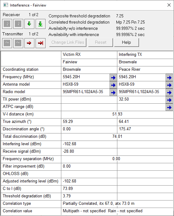
Position the Interference dialog so that the selected receiver is visible on the network display. Each interference sub case will be graphically displayed.

In the example header above, there are two receivers at Site D. The coordinating station for receiver 1 is Site C. There are three transmitters interfering with receiver 1. The overall results for this receiver are summarized as follows:

The composite threshold degradation due to all interfering transmitters.
The composite threshold degradation considering the correlation status of the interfering transmitters. The correlated threshold degradation is shown for both multipath and rain.
The one way link availability at the receiver without interference,
The one way link availability at the receiver with the composite correlated interference

Click the red arrows to step through the interfering sub cases for the selected receiver.

Click the green arrows to step through the receivers at this site

The following data is displayed for each interference case:

Frequency and polarization of the receiver and interfering transmitter
Antenna model of the receiver and interfering transmitter
Radio model of the receiver and interfering transmitter
Interfering transmit power
Interfering transmitter ATPC range
Distance between the receiver and interfering transmitter
True azimuth of the of the receiver and interfering transmitter antennas
Total discrimination of the receiver and interfering transmitter antennas
The level of the interfering signal at the receiver
The receive signal level from its coordinating station
The frequency difference between the receiver and the interfering transmitter
The filter improvement due to the frequency and bandwidth difference between the receiver and the interfering transmitter
The over the horizon loss (OHLOSS) for an interfering path which is not directly connected to the receiver
The adjusted interfering level including the filter improvement and the OHLOSS
The carrier to interference ratio (receive signal to adjusted interfering level)
The threshold degradation
The type of correlation
The specified correlation values for multipath and rain

Changing Parameters

The following parameters can be changed for the receiver

Frequency and polarization
Receiver antenna
Receive radio

The following parameters can be changed for the interfering transmitter

Frequency and polarization
Transmit antenna
Transmit radio
Transmit power
Transmit ATPC range

Click the blue arrow for the parameter to be changed. The associated data entry form will appear. The interference results will be automatically be recalculated and displayed. The Reset button and the Change Link Files button will become active whenever a change has been made.

Reset

This will reset all interference cases to the values on entry. Any changes made to any case or sub case will be lost.

Change Link Files

The associated link design files are not modified during the interactive procedure. Click the Change Link Files button to incorporate the changes to the individual Link design files. This operation will erase the main interference calculation and close the Interference dialog

Other Considerations

When a change is made and the interference is recalculated, OHLOSS calculations are not recalculated. The original values are used. If the changes made result in a new OHLOSS case, the case will not be valid.

If an OHLOSS case has not been calculated, the case will be marked as not calculated in red. In these cases it is necessary to return to the main interference calculation and either repeat the calculation using the Calculate OHLOSS automatically or carry out the calculations in the case detail interference report

Changes to the frequency, polarization, ATPC use the standard Frequency assignments data entry form. If multiple channel assignments have been made, it is users responsibility to change the parameters for the specific case or sub case. Additional channel assignments should not be added.

In the Change Pl5 files operation, any changes to a radio will be carried out at both ends of the link for point to point links. In point to multipoint links, only the change will only be made at the base station or remote as applicable.

Interference Calculations using the MDB

The Intra System Interference dialog contains a special group “MDB sites” in the Study Scope group box. The Study Scope “Analyze MDB sites against MDB sites” is not allowed.

The arrow between the analyze and against groups denotes the direction of the calculation. Click on the arrow to change between a single direction and a bidirectional calculation.

Analyzes the interference from Network display transmitters into MDB receivers. In order do the interference calculation in the opposite direction, reverse the groups in the study scope.

The interference analysis is carried out in both directions.

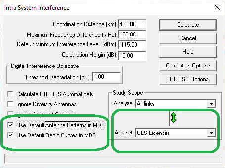
Default Antenna Patterns in MDB

The interference calculation includes an option to use default antenna patterns if an antenna code is not specified. The default is based on the antenna beam width and frequency. If the beam width is not available, it will be calculated from the antenna gain and the frequency.

Default Radio Curves in MDB

The interference calculation includes an option to use default radio curves in interference calculations when using a MDB.

If the radio data includes an emission designator, the bandwidth will be extracted and used to generate default transmit emission and receiver sensitivity masks.

FCC ULS Database

Pathloss 6 includes support for the FCC ULS Database. Users working in North America can download the FCC’s ULS data and use it in Pathloss to perform interference calculations against Pathloss designs. This feature is only available with the Interference option.

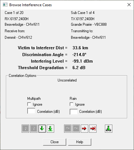
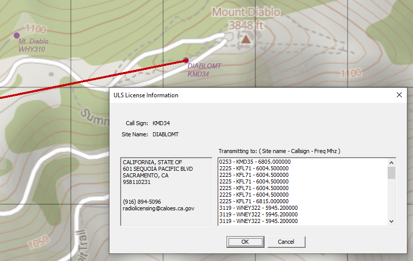
Licenses requiring coordination are displayed graphically in the new Browse Interference cases window. The NSMA defined coordination area is displayed along with the stations that met the interference objective. The user can toggle though the cases and sub cases and the interfering path is displayed. Users can click on an interfering site, and the site details are displayed. The the following information is displayed:

Site name
Callsign
Owner details and contact information
All coordinating stations for the license

The download process is fast and simple using the dedicated ULS Data Download (UDD) program. New License data is published every Sunday on the FCC website.

Instructions for use

Download the Data

Download the data using the ULS Data Download (UDD) program. This program is located in the Pathloss 6 folder in the Start menu.

Click Download ULS and the data will be downloaded and converted.

Configure Pathloss to use FCC ULS Database

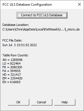
Configure Pathloss to use the data by clicking Interference-Database-Configure FCC ULS Database in the main window.

Clicking the Connect to FCC ULS Database will automatically open the default database location. Select the l_micro.uls data file and click Open. Some information about the table is displayed and the table is now ready for use.

Using the FCC ULS Database in an Interference Calculation

To use the data in a calculation, select ULS Licenses from the choices in the Against drop-down list. The Use Default Antenna Patterns in MDB and Use Default Radio Curves in MDB option will also need to be checked.

Graphically Browsing Interference Cases

Once the calculation is complete click Interference-Browse Interference Cases. The green up and down arrows toggle between cases and the red left and right arrows toggle between sub-cases.

The ULS sites are shown in purple in the display. The user can click on a site to pisplay more information.

Interference Reports

Summary Report

This report provides a listing of the report case with the minimum of detail. An example of this report is shown below:

Case 1 ES01 from NS01 - 5863.125H - threshold degradation 2.23 dB 1-1 NS01 to NS02 - 5863.125H - correlated case V-I distance 42.43 km interfering level -103.03 dBm threshold degradation 5.53 dB 1-2 NS03 to NS02 - 5863.125V - OHLOSS case V-I distance 131.96 km interfering level -122.92 dBm threshold degradation 0.11 dB

Cross Reference Report

This report provides a concise summary of the interference cases. It is intended to be used as a cross reference into the case detail report. An example of this report is shown below:

Coordination distance(km) 200.00 obj Objective (dBm) Maximum frequency separation(MHz) 150.00 v-i V-I distance (km) Default minimum interference level(dBm) -115.00 tad Total discrimination (dB) Margin(dB) 10.00 ifl Interfering level (dBm) Threshold degradation objective(db) 1.00 td Threshold degradation (dB) Total number of cases calculated 12 _mp _rn multipath - rain correlated OHLOSS case * Correlated case ** Case 1 ES01 (NS01), 5863.125V, HPX8-58W-TR, 6706-8, obj = -113.0, td_mp = 8.6, td_rn = 9.3 1-1 NS01 (ES01), 5878.875V, HPX8-58W, 6706-8, v-i = 42.4, tad = 0.0 (i 0.0° v 0.0°), ifl = -99.5 (-13.5), td = 8.36 ** 1-2 NS01 (NS02), 5863.125V, HPX8-58W, 6706-8, v-i = 42.4, tad = 67.0 (i 165.8° v 0.0°), ifl = -105.0 (-8.0), td = 4.19 * Case 2 ES01 (NS01), 5878.875V, HPX8-58W-TR, 6706-8, obj = -113.0, td_mp = 9.2, td_rn = 9.8 2-1 NS01 (ES01), 5863.125V, HPX8-58W, 6706-8, v-i = 42.4, tad = 0.0 (i 0.0° v 0.0°), ifl = -98.7 (-14.3), td = 9.01 ** 2-2 NS01 (NS02), 5878.875V, HPX8-58W, 6706-8, v-i = 42.4, tad = 67.0 (i 165.8° v 0.0°), ifl = -105.1 (-7.9), td = 4.17 **

Case Detail Report

The case detail report provides the highest level of detail on the interference cases. This report allows the following operations:

View the TX and RX antenna specifications
Views the TX and RX radio specifications
Modify or ignore an interference case
Calculate OHLOSS for a given case
Delete an interference case and all sub-cases or a sub-case only

A sample report is show below:

Case 2 - ES01 from NS01 Victim RX Interfering TX ES01 NS01 Latitude 55 48 09.00 N 56 05 29.88 N Longitude 120 12 58.00 W 120 12 58.00 W True azimuth(°) 40.46 55.03 Coordinating station NS01 NS02 Antenna model HPX8-58W HPX8-58W Usage TR TR Antenna file name 1992 1992 Antenna height(m) 6.59 74.33 Antenna gain(dBi) 40.80 40.80 Polarization Vertical Vertical Discrimination angle(°) 0.00 165.79 Radio model MDR-6706-8 MDR-6706-8 Radio file name 6706-8 6706-8 RX - TX loss(dB) 2.22 5.75 TX power(dBm) 29.00 ATPC range(dB) RX noise floor(dBm) -107.13 Frequency(MHz) 5878.8750 5878.8750 Channel ID 6l 6l V-I distance(km) 42.43 V-I free space loss(dB) 140.41 V-I atmospheric absorption loss (dB) 0.28 Antenna discrimination(dB) HH HV VV VH Interfering TX 65.00 69.00 67.00 69.00 Victim RX 0.00 32.00 0.00 32.00 Total discrimination(dB) 65.00 69.00 67.00 69.00 Interfering level(dBm) -103.05 -107.05 -105.05 -107.05 Performance degradation Objective(dBm) -113.00 Receive signal(dBm) -35.53 Interfering level(dBm) -105.05 Frequency separation(MHz) 0.00 Filter improvement(dB) 0.00 Other loss(dB) Adjusted interfering level(dBm) -105.05 C to I(dB) 69.52 Threshold degradation(dB) 4.17 Partially correlated - MP 6.0, RN 0.0 dB

Hi-Lo Violation Report

This report simply provides a listing of all transmit frequencies used in the interference analysis. The channel ID letter (H or L) is used as the high low consistency check. All frequencies at a site must be either H or L or a high low violation exists which is sometimes referred to a frequency buck. The interfering effect is best determined by actual site measurements.

TX RX ES01 NS01 5896.625V C03H NS01 5912.375V C06H NS01 ES01 5863.125V C03L NS02 5878.875V C06L NS02 5863.125V C03L ES01 5878.875V C06L NS02 NS01 5912.375V C06H NS01 5896.625V C03H NS03 5912.375H C06H NS03 5896.625H C03H NS03 NS02 5863.125H C03L NS02 5878.875H C06L