Local and Area Studies

Basic Concepts

A study calculates the receive signal strength from a base station over a user defined region. In a local study, each base station has its own circular region centered on the base station. In an area study, there is only one region which can be a circle, rectangle or a polygon and can be positioned anywhere on the display. The signals from all base stations are calculated into this common region.

From this definition, it is apparent that a local study can only display received signal levels. If several local studies overlap, then the strongest signal will be displayed.

In the case of an area study, the signals from each base station are available in the common area; and therefore, the analysis can be extended to include:

• Most likely server
• Carrier to interference
• Simulcast delay spread

Study Extents and Resolution

The first step in a local or area is to define the study extents. In the case of a local study, the user simply specifies the radius. In an area study, the user defines a circle, rectangle or polygon, positioned in the region of interest on the display.

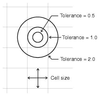The second step is to define the resolution and tolerance for the study. The user specifies a cell size and the region is divided into rows and columns of square cells. A calculation will be made for each cell. There are practical limits for the resolution (cell size) and depending on the overall dimensions of the region, memory allocations may fail.

The tolerance is a measure of the calculation detail. A tolerance of 1 means that if a circle is drawn at the center of a cell with a diameter equal to the cell size, then there will a calculation point somewhere inside this circle. If the tolerance is 0.5 then the diameter of the circle containing a calculation point will be 0.5 * cell size. Note that the tolerance can be greater than 1. For a tolerance of 2, the radius would be 2 * cell size and the same calculation point would be used for several cells.

A tolerance (T) guarantees that a path profile will be available for each cell at a point not greater than T*cell size /2 from the center of the cell. At points near the base station, the radial density is high. The limiting values occur at the extremities of the study where radial density is at its minimum.

The tolerance determines the number of profiles required for each base station. As an example, consider a local study with radius of 25 kilometers and a cell size of 100 meters. The number of profiles required for several tolerance values is given below.

• A tolerance of 0.1 requires 12,240 profiles
• A tolerance of 0.5 requires 2808 profiles
• A tolerance of 1.0 requires 1452 profiles
• A tolerance of 2.0 requires 746 profiles

Profile generation is the most time consuming part of a study calculation. In the interests of calculation time, preliminary studies should not use a tolerance less that 1.

GIS Configuration Considerations

A terrain database must be setup in the GIS configuration. Before starting the calculation, select the Configure - Program options - Terrain Data - Profile generation to verify the database settings.

Primary and Secondary DEMs

If the terrain elevation data has bad or missing data, then the radial profile generation will stop at the first bad data point encountered. The segment of a local study display shown on the right was generated with SRTM data. The white portions of the display represent missing data. The calculation will be missing from the start of this missing data to the edge of the study extents.

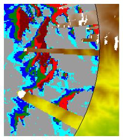
When this situation is encountered, one solution would be to configure a secondary database in the GIS configuration. If the missing data patches are random and relatively small, then GTOPO30 would be a reasonable candidate for the secondary database.

Note that local and area studies cannot detect any changes to the primary or secondary DEMs or the clutter databases. In order to recalculate the studies, check the Force recalculation option.

Clutter Loss Calculations

Clutter databases fall into two general categories:

• The clutter database contains the actual clutter heights at each point on the profile. No other information is available. Note that this type includes the clutter derived from the differential elevations between two databases such as SRTM and NED
• The clutter database only contains a description of the clutter. The user has assigned heights to be used for each clutter type. In addition, each clutter type in the database is cross referenced to a set of standard clutter categories. These standard categories, in turn, define the clutter loss versus frequency and the standard deviation of the log normal probability distribution used to calculate location variability.

In all cases, the program calculates the diffraction loss from the base station to the specific cell in the study using the terrain DEM. This base calculation does not consider clutter heights.

In the first case, where the clutter elevations are in the database, the incremental clutter loss is calculated and added to the above diffraction loss. The basic algorithm for this calculation is an effective knife edge and is defined in detail in the diffraction technical reference. The user specifies a default clutter category which in turn sets the log normal standard deviation for location variability. This correction is applied to all cells.

In the second case, the method depends on the mobile antenna height relative to the clutter height. If the mobile antenna height is over the top of the clutter, then the above method is used; otherwise the following procedure is used:

• a 200 meter exclusion zone is setup at the mobile end of the profile
• The loss due to clutter on the path profile from the base station to the edge of the exclusion zone is calculated both as an effective knife edge and as lateral wave or multipath propagation for trees and buildings, respectively. The loss due to clutter on the profile is assigned the smaller of the two values.
• In the immediate vicinity of the receiver (inside the 200 meter exclusion zone), the loss is determined from the loss versus frequency table for the specific clutter category in the cell.
• This loss is then scaled based on the mobile antenna height relative to the clutter height from zero at the clutter height to the full value at the mid point of the clutter height.
• The clutter loss on the profile and the loss in the exclusion zone are both added to the path profile diffraction loss.

The log normal standard deviation for the specific clutter category in the cell is used for location variability.

Display Projection

The network display uses a rectangular projection to display the sites and links. The specific projection is determined from the following priorities in the GIS configuration:

• If the network display includes backdrop imagery including geo-referenced images, then the backdrop projection will be used.
• If vector files using a non geographic projection are included, then the vector projection will be used
• If the sites projection is set to a non geographic fixed zone projection then this projection will be used
• The default is a transverse Mercator projection with the central meridian set to the mid point of the east - west extents of the display.

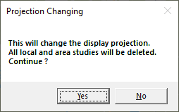
When a local / area study is created, the rows and columns which define the cells are based on the current network display projection. If this is changed for any reason, all study displays become invalid and will be erased.

An example of how this situation may arise is now described. The network display is using the default transverse mercator projection and a study is created. The central meridian of this transverse mercator projection is now fixed. If new sites are added which change the east west extents of the display, this would normally reset the central meridian. When a local or area study is defined, this change will have no affect on the projection.

The user now decides to add an aerial photo to the display. The photo is in a tiff file and uses a UTM projection. The error message shown on the right will appear.

Be sure to include all required backdrop imagery before creating the study.

Display Criteria

Local and area study displays are color coded to represent signal levels. The selection of the criteria, range and color coding is made using the color ramp control. This control is used throughout the Pathloss program and a complete description is given in the help section on General program operation.

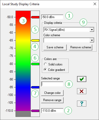
The color ramp shown on the left is a partial representation of the display criteria color ramp with numbers on various key components. These numbers will be used in the following setup instructions:

• Select the display criteria from the drop down list (9).
• Enter the maximum value (1).
• Enter the minimum value (2).
• To change the color of a range, double click on the display range at (3) or double click on the range marker (4).
• The top and bottom range markers are fixed. To move any other range marker, hold the left mouse button down on the marker (6) and raise or lower it to the new location. You can cross over an existing range marker. Be careful not to move the mouse out of the range marker column, as this will delete the range (7).
• A range can also be moved by entering its new location in the selected range (8). Click on the range marker to be moved (4). Its position will be displayed in the selected range (8). Enter the new value and press the tab key or click on another location, The range will be updated when the selected range edit control loses focus.
• To add a new range, double click on any blank area in the range marker column (5). The default color for the new range will be the same as the previous range. Double click on the new range marker and set the color for the new range.
• To delete a range, hold the left mouse button down on a range marker and drag the mouse out of the range marker column (7).

The following display criteria are available for both local and area studies.

• Receive signal - dBmV
• Receive signal - dBm
• Receive signal - dBW
• Receive field strength - dBmV/m
• Fade margin - dB
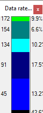
• Data throughput

The data throughput criteria is only available in adaptive modulation applications. The base station and remote must include a radio data file with the adaptive modulation section completed. The ranges will be automatically set to the receive threshold levels and the vertical axis will display the corresponding data throughput. The ranges cannot be edited. Only the colors can be changed.

The local study also includes a line of sight display. The area study includes the following additional display criteria:

• Most likely server
• Carrier to interference
• Simulcast display spread

Details on these display criteria are given in the Local study and Area study sections respectively.

Path Profile Generation

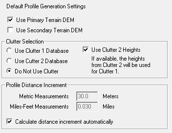
These options specify the usage of the primary and secondary DEMs and the clutter model selection for profile generation in local and area studies. These are the basic program options and are repeated here to the allow the user to compare the results for different GIS configurations.

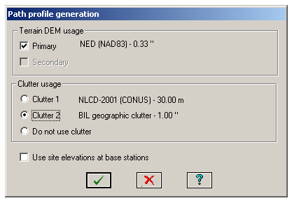
In the network display, these options are accessed from the Configure - Options - Program options - Terrain Data - Profile generation.

Normally all path profile elevations are taken from the primary or secondary DEMs. An option is provided to use the elevation specified in the site list for the base station elevation.

Use Site Elevations at Base Stations

The following points should to be considered for the Use site elevations at base station option.

Calculations such as antenna heights, clearance and diffraction loss are based on the clearance to first Fresnel zone ratio. In these calculations, all elevations are relative to the end point elevations. The absolute elevations above mean sea level are not used. In other words the entire profile could be shifted up or down with no change to the results.

Therefore, the absolute error in the elevations has no significance in the calculations. It is the relative errors (the elevation differences between the end points and the critical points on the profile) which make the difference. Changing the site elevations has the same effect as changing the antenna heights.

The type of terrain database must be considered. These can be divided into two classifications for the purposes of this discussion - bare earth and composite terrain and clutter. NED data is an example of the first and SRTM is an example of the second type. In the case of the composite terrain and clutter database, the elevations may include some degree of structure heights and the site ground elevations should be used at the base station. In all other cases, the accuracy of the site elevations and the resolution of the terrain database will determine the choice.

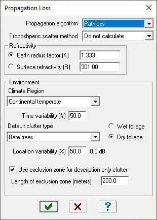Propagation Parameters

These setting define the algorithms to be used in local and area studies. If the Propagation algorithm, Tropospheric scatter method or Refractivity settings are changed, a complete recalculation including terrain profile generation is required. Changes to the Environment settings only require a signal recalculation.

Propagation Algorithm

Choose either the Pathloss or Tirem algorithms. The NSMA algorithm is intended for the analysis of interference paths.

Refractivity

Specify either the effective earth radius factor K or the surface refractivity at the base station.

Climate Region

This climate region determines the statistical dataset to be used to calculate the time variability for time percentages greater than 50%.

Default Clutter Type

The clutter category is used to calculate the clutter loss on a path profile. In a description only database, the actual clutter category at the location will be used. In all other cases, the default clutter category will be used over the complete profile. If the default clutter is not one of the building types, then it is necessary to check the Wet or Dry foliage option.

Wet - Dry foliage

This option applies to the default clutter category and all the tree type clutter categories in a description only clutter database. This option can have a significant impact on clutter loss.

Location Variability

The clutter category determines the standard deviation of a log normal probability. This is used as the basis of the location variability for time percentages greater than 50%.

Use Exclusion Zone for Description only Clutter

This option applies to description only clutter databases and is only used in local and area studies. If the clutter height at the mobile location is greater than the antenna height, then the clutter within 200 meters of the mobile will not be considered in the profile clutter loss calculation. To account for the clutter loss in the immediate vicinity of the mobile, a loss based on the frequency and clutter type is added. These losses are defined in the clutter GIS configuration. If the mobile antenna height is greater than 0.5 of the clutter height, the loss will scaled to 0 dB at the clutter height.

If this options is not checked, the clutter loss will consider all clutter on the path profile as is the case for all link calculations.

Tropospheric Scatter Method

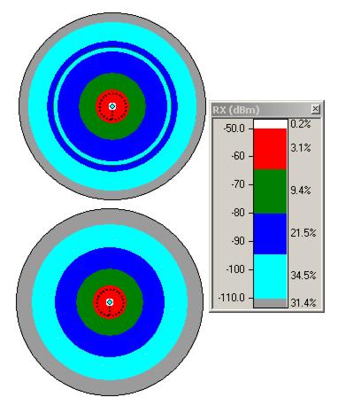
The local study display on the right shows the effects of tropospheric scatter on an over water area using an omnidirectional antenna.

In the top display, tropospheric scatter is enabled. The signal decreases with distance until tropospheric scatter becomes the dominate propagation mechanism and the signal will increase for a certain distance before decreasing again.

In the bottom display, the Tropospheric scatter method is set to Do not calculate. The signal simply decreases with distance as expected.

Note that the coverage area will be slightly better when using tropospheric scatter.

In marine applications, it may be advantageous to present both scenarios as a best - typical case comparison.

In all other applications, the Tropospheric scatter method should be set to Do not calculate.

Location and time variability

The base diffraction - tropospheric scatter calculations are valid for 50% of the time and 50 percent of all locations. The user can enter higher time percentages in the range from 50 to 90% for the location and time variability. The effect will always be a reduction in the coverage area.

The probability distribution for time variability uses an empirical relationship based on frequency, climate region and the effective path length. Details of this algorithm are given in the Diffraction Technical Reference chapter.

Location variability is calculated using a log normal probability distribution. The standard deviation is determined by the clutter category in each cell of the study if a “description only” clutter database is used. In all other cases, the default clutter category will be used for the standard deviation and the additional loss shown will apply to all cells.

Basic Local and Area Study Calculation

Path profiles are created from the base station to each cell in the study. The following parameters are calculated for each profile:

• Path length
• Free space loss
• Diffraction loss
• Clutter loss
• Vertical angle at the base station. The overall base station antenna orientation loss considers the base station sector azimuth, mechanical down tilt and the vertical angle. Mobile antennas are assumed to be perfectly oriented at the base station.
• Effective path length. This parameter is used to calculate time variability.
• Clutter category. This determines the log normal standard deviation to calculate location variability.

This step is the most time consuming part of the calculation. The results will be invalidated if the extents or resolution of the study, frequency, antenna heights, K, or the diffraction algorithm are changed.

The calculated data is saved in a file named after the base station and the site id with the file suffix “lsy” for local studies and “asy” for area studies. These files are located in the network gr5 file directory and will be used for all subsequent signal level calculations. Any changes to equipment parameters such as the transmit power and antenna gain or the display criteria can be rapidly recalculated.

Receive Signal Strength (RSS) calculations

In a local study, the RSS is calculated in each cell of the study. In an area study, the RSS is calculated for each base station in each cell of the area display. The display criteria can be set to the following units

• RX Signal (dBmV)
• RX signal (dBm)
• RX signal (dBW)
• RX field strength (dBmV/m)
• Fade margin (dB)

The calculation procedure for each cell is summarized below:

• Calculate the azimuth from the base station to the cell. The mobile antenna in the cell is assumed to be perfectly oriented to the base station.
• Determine the sector number for this azimuth.
• Calculate the horizontal angle between the sector azimuth and the azimuth to the cell.
• Calculate the base sector antenna discrimination from the horizontal angle, the vertical angle and the antenna downtilt.
• Calculate the basic transmission loss (BTL) as follows:

BTL = free space loss + diffraction loss + clutter loss - base antenna gain - mobile antenna gain

In the downlink direction (mobile receive and base station transmit)

RSS = BTL + base sector tx power - base sector tx loss - base sector antenna discrimination + mobile rx loss

In the uplink direction (base station receive and mobile transmit) the receive signal is given by:

RSS = BTL + mobile tx power - mobile tx loss - base sector rx loss - base sector antenna discrimination

In the case of non symmetrical sectors, the above calculation sequence is carried out for each base station sector and the maximum value is used.

Base Stations

Base stations are used in point to multipoint link design, local and area studies. The first step in these operations will be to create a base station. Any site on the network display can act as a base station; however, there can only be one base station at a site. The site retains its normal point to point functionality.

A base station definition includes both the base and remote site specifications.

When a base station is first created or edited, it becomes a template for the next base station to be created. This template does not include the base station antenna height or the specific sector frequency assignments.

Base Station Creation

In some operations such as point to multipoint link design and local studies, the base station definition is included in the design procedure. A base station can be created at a single site or multiple base stations can be created for a group or selection of sites.

To create a single base station, right click on the site legend and select the Base station - Create edit menu item.

To create multiple base stations, first create a selection or group of sites and then select the Studies - Base stations - Create menu item on the network display menu bar.

If this is the first base station in the network display, then the default calculation options (application type and frequency) will be applied to the base station, otherwise the base station template will be used.

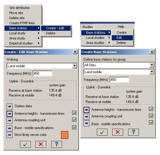
If necessary, set the Application type (microwave, adaptive modulation or land mobile) and the design frequency.

The system gain is shown for the uplink and downlink transmission directions. This is defined as the difference between the transmit power and the receive sensitivity plus the sum of the antenna gains, and minus the transmission line and antenna coupling unit losses. The worst transmission direction (lowest system gain) is usually selected for the analysis. The values will not be available if the base - mobile specifications are incomplete.

The following data entries are required to create the base station:

• Station data (call sign, station code, operator code). These are optional entries and are only available for base station creation at a single site.
• Antenna heights and transmission lines
• Antenna coupling unit
• Base station - mobile equipment specifications

Most likely server color

The most likely server color is used in area studies. The default color is the site legend color. Changing the most likely server color also changes the site legend color.

Antenna Heights

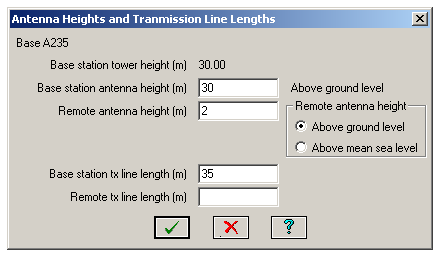
Both the base station and remote station antenna heights must be specified. The base station antennas height is always measured from ground level. The mobile antenna height can relative to ground level or to sea level. The sea level reference is intended for aircraft to ground station analysis.

If transmission line losses are to be included, specify the transmission line lengths for the base and remote stations.

The equipment specifications section contains the transmission line specifications.

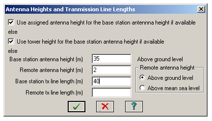
When multiple base stations are being created, an option is provided to set the base station antenna height to:

• The assigned antenna height if available
• The tower height if available.
• The specified antenna height

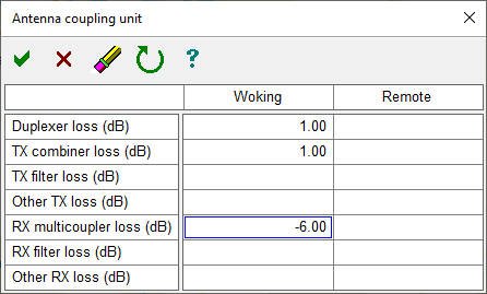
Antenna Coupling Unit

Click the Antenna coupling unit button to access the data entry for the base station and remote. In land mobile applications, the RX Multicoupler loss can be a negative number which implies gain.

 

Base - Mobile Equipment Specifications

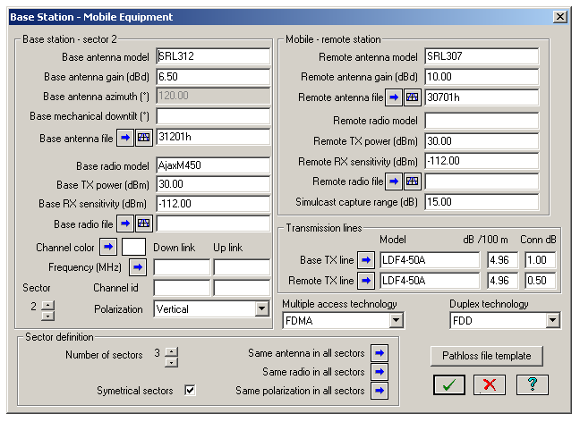
The base mobile equipment specifications can be accessed from either:

• The Link design rules in a point to multipoint design. Click the Equipment specifications button.
• The Create base station dialog in a local or area study. Click the Base - mobile specifications button.

These specifications apply to the selected base station and the remote / mobile site. Base station equipment specifications are saved in the network gr5 file and not in the link design rules (ld5) file. The data entry is organized in the following sections:

Base station sector data

A base station can have a maximum of 8 sectors as set in the Sector definition group box. Each sector contains the antenna and radio data and its frequency assignment. Multiple sectors can be symmetrical or non symmetrical as determined by the Symmetrical sectors check box.

 In the symmetrical case, only the azimuth of the first sector can be set. The azimuths of the remaining sectors will be automatically set and are shown as the pie diagram on the left. In the non symmetrical case, the azimuth of each sector must be set. These are shown as arrows in diagram on the right. The sector colors in these diagrams correspond to the frequency assignments. A dotted black line denotes that frequency assignments have not been made. When specifying multiple symmetrical sectors, always complete the data entry for sector 1 first. When sector 2 is selected the first time, the sector 2 data will default to the sector 1 data.

Note the following points concerning the data entry:

Sector antenna data

• For a single sector base station antenna, it is sufficient to simply enter the antenna gain in the units shown (dBd or dBi as determined by the design frequency). In this case, an omnidirectional horizontal antenna pattern will be used with no provision for the vertical angle antenna discrimination.
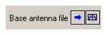•  An antenna data file is required to include the base station antenna pattern in the analysis. Click the Base antenna file button to add an antenna from the index. If this is a directional antenna, then enter the azimuth, and optionally, the antenna mechanical downtilt. The second button on this line provides a view of the antenna specifications and patterns.
• An antenna data file is required if the base station is included in an interference calculation.
• Antenna data files are required for multiple sectors. For symmetrical sectors, the 3 dB beam width should correspond to the number of sectors. For example for three symmetrical sectors, 120 degree beam width antennas would be used.
• For non symmetrical sectors, the analysis determines the antenna gain from each antenna at the particular azimuth and uses the maximum value.
• To set the antenna data in all sectors to the data in the selected sector, click the Same antenna in all sectors button. This is useful if an antenna model is changed.

Sector radio data

• The basic radio data requirements are the transmit power and the receiver sensitivity. Click Base radio file button to add a radio data file from the index. The second button on this line provides a view of the radio specifications and curves.
• A radio data file is required for adaptive modulation applications (OFDM - WIMAX). In this case the transmit power and receive sensitivity for the highest modulation level are shown when the radio data file is loaded.
• A radio data file is also required if the base station will be used in an interference analysis.
• Click the Same radio in all sectors button to set the radio data in all sectors to the data in the selected sector. This is useful if the radio model is changed.
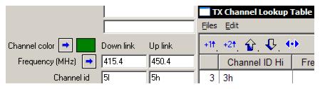•  Frequency assignments are required for an interference analysis. The TX channel lookup table can be used as shown in the excerpt on the right. Click the Frequency (MHz) button to bring up the table. The up and down arrows change the sector number. The +1 and +2 buttons copy the high frequency to the base station or remote station, respectively.
• As a visual aid in the network display, the sectors can be color coded for their frequency assignment. Click the Channel color button and select the desired color.
• Set the polarization for each sector using the drop-down list. To set the polarization in all sectors to the value in the selected sector, click the Same polarization in all sectors button.

Mobile - remote antenna and radio data

The basic data entry requirements are the antenna gain expressed in dBi or dBd as determined by the design frequency and the transmit power and receiver sensitivity.

If the remote antenna, is not omnidirectional, an antenna data file is required for an interference analysis. In a carrier to interference analysis, the remote station antenna is oriented to the base station with the highest signal. The antenna discrimination to all other base stations is calculated using the antenna data file. Click the Remote antenna file button to access the antenna index and select the antenna data file.

A radio data file is required for an interference analysis which requires frequency discrimination data. Click the Remote radio file button to access the radio index and select the radio data file.

Transmission lines

If the design scope includes Add TX line data, enter the transmission line, model, unit loss and optionally, the connector loss. Click the Base TX line or Remote TX line button to access the transmission line table. The connector loss for the base and remote stations can also be entered here.

Duplex and multiple access technology

The calculation of the composite interfering signal depends on the duplex and multiple access technology used in the radios. The duplex technology can be frequency or time division duplex - synchronized or non synchronized.

There are three options for duplex technology, and five options for multiple access technology. The technology is applied to every sector in the base station. The effect of each technology is explained below:

Duplex Technologies

Frequency Division Duplex (FDD)

Both the base station and the remote stations transmit at the same time using different frequencies. All transmitters are considered in interference studies.

Time Division Duplex (TDD non synchronized)

The base station and the remotes use the same frequency. Only the base station or one remote station can transmit at a time. Therefore, in an interference study, only the worst case (between the base station and the combination of remote stations) is taken in each sector.

Time Division Duplex (TDD synchronized)

This is a specialized form of duplexing between separate base stations. Base stations are synchronized with one another so that corresponding sectors will not be transmitting at the same time. There will be no interference cases between same numbered sectors of base stations using this technology.

Multiple Access Technology

Time Division Multiple Access (TDMA)

Only one remote per sector is transmitting at any time. Only one remote per sector is considered in interference cases. This will be the remote causing the worst interference.

Frequency Division Multiple Access (FDMA)

All remotes are transmitting simultaneously. All Interference cases are considered.

Code Division Multiple Access (CDMA)

All remotes are transmitting simultaneously. All Interference cases are considered. Power levels for remotes are adjusted so that the receive signal power at the base station from each remote is equal.

Orthogonal Frequency Division Multiple Access (OFDMA)

All remotes are transmitting simultaneously. All interference cases are considered.

Carrier Sense Multiple Access (CSMA)

This is also referred to as contention and is a form of TDMA. The mobile transmission is inhibitted if another remote is transmitting thererby preventing a collision. In the program, it is handled in the same manner as TDMA..

Edit Base Stations

To edit a base station at a specific site, right click on the site legend and select the Base station - Create - edit menu item.

To edit multiple base stations, first create a group of sites with base stations. This group must not contain any sites without base stations or the operation will fail.

Select the Studies - Base stations - Edit from the network display menu bar.

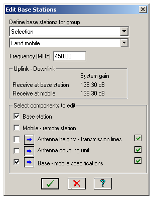
Note that check boxes are provided for restricting the editing operations.

Both the base station and the mobile station can be edited. At least one of these must be checked.

The Antenna heights - transmission lines, Antenna coupling unit and the Base - mobile specifications can be edited. At least one of these categories must be checked.

All other aspects of the Edit base stations procedure are the same as the Create base stations procedure.

The edit operation will invalidate any local studies or an area study involving the group of base stations. If the Antenna heights - transmission lines option is checked, this will be interpreted as an antenna height change. This will result in a complete recalculation including profile generation. If the Antenna coupling unit or Base-mobile specifications are checked, then only the signal strength will be recalculated.

To delete a single base station, right click on the site legend and select the Base station - Delete menu item.

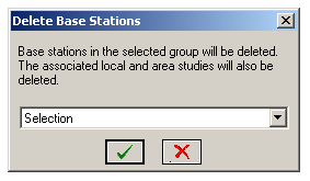
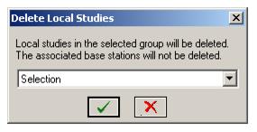
A group or selection of base stations can be deleted. Local studies and an area study associated with these base stations will also be deleted. Select the Studies - Base stations - Delete from the network display menu bar.

Local Study

Overview

A local study can be created at any site in the network display. If a base station does not exist at the site, one will be created as part of the procedure. In this case, the study radius can be different at each base station.

Additionally, local studies can be created for a group of existing base stations using the same radius at all base stations.

The following parameters are common to all local studies:

• Display criteria
• Propagation parameters
• Receive at mobile or base station (down link - up link)

If any of these parameters are changed for one study, all local studies will be reset to these values and recalculated. In the case of propagation parameters, this will involve a complete recalculation including path profile generation.

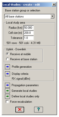
Creating a Local Study at a Site

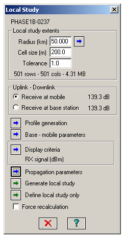
To create a new local study or to edit an existing one, right click on the site legend and select the Local study - Create /edit menu item and follow the procedure below:

• Specify the radius for the study. Alternately, click the Radius button. Move the cursor on to the network display. The cursor will change to a measurement cursor. Click on the display to define the radius. A circle will be drawn around the site. When the desired radius is set, click anywhere on the Local study dialog to reset the cursor.
• Specify the Cell size and Tolerance.
• If a base station has not been defined or needs to be edited, click the Base - mobile parameters button.
• Select the Uplink - Downlink transmission direction. The system gain in each direction is shown.
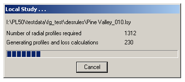
• Click the Generate local study button to run the calculation now. Note that any other existing studies which have modified data will also be generated at this time. Click the Cancel button to terminate the calculation
• Alternately, click the Define local study only button to just define the study and exit the dialog. This allows all studies to be generated in one calculation run.

The program tracks changes to parameters which affect the local study. If the study is invalidated due a parameter change, it will be erased leaving only the circle outline. However, if changes are made to the GIS configuration e.g. adding a clutter database, it will be necessary to check the Force recalculation option and then click the Generate local study button.

Creating Local Studies for a Number of Base Stations

Local studies can be created for a group of base stations using the same radius for all studies. Complete base station definitions are a prerequisite for this operation.

Create a group or selection of base stations. The default “All base stations” item will check for a base station at each site in the Network display. Select Studies - Local studies - Create - edit. The basic procedure is given below:

• Enter the study Radius, Cell size and Tolerance.
• Specify the direction of transmission - Receive at mobile or Receive at base station.
• If necessary edit the Propagation parameters.
• Click the Generate local studies button to run the calculations now or click the Define local studies only button to run the calculations later.

Line of Sight Display Criteria

In addition to the signal strength display criteria described in the Basic concepts section, the local study includes a Line of sight display criteria. This is not a free space line of site test. Fresnel zone clearance is not included in the analysis. A grazing path would pass this line of sight test. The specified value of K or surface refractivity is included.

Set the visible and shadow colors. The transparency of the colors can be set to show the backdrop imagery, elevation and clutter displays.

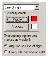
Two visibility definitions are available in overlapping areas:

• If a point in the overlap area is visible to Any site, it is marked visible.
• If a point in the overlap area is visible to Every site, it is marked visible.

 The latter definition is useful to find all areas which are visible to two or more sites. The diagram on the right shows two line of sight local studies using the Every site visibility option. In the overlap area, the red areas represent locations which have a grazing path or better to both sites.

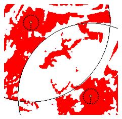
The remote site antenna heights at both sites must be set to the same value. This height could be a tower height limit for the new site.

Local Study Visibility

The entire Network local study display can be switched on and off using the View - Extents - layers menu item. Click the Local study check box in the Layers group box.

A single local study can be switched on and off in the Site list. Click the check box in the Show local study column for that site.

To delete a local study at a site, right click on the site and select the Local study - Delete menu item.

To delete a group or selection of local studies, select the Studies - Local studies - Delete menu item.

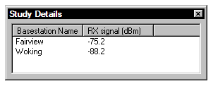
View Study Details

Select the View - Study details - Local studies menu item to view the calculated signal strengths from all base stations at the mouse cursor location.

Area Study

In a local study, each base station has its own study area i.e. the circle around the base station. There can be as many local studies as there are base stations. An area study, on the other hand, has one common area in which signal levels are calculated from all base stations. This means that there can only be a single area study in the network display.

The display criteria can be any of the receive signal strength options available in local studies, plus the following displays which are applicable to area studies only:

• Most likely server
• Carrier to interference
• Simulcast delay spread

All base stations must be defined in advance to create an area study. The base station definition is exactly the same for a local study or an area study.

Create Area Study

Select the Studies - Area studies - Create edit menu item on the network display menu bar.

Note that the analysis can be carried out for all base stations, a temporary selection of base stations or a defined group of base stations. The base station symbol for any base station which is not part of the area study will be colored dark grey.

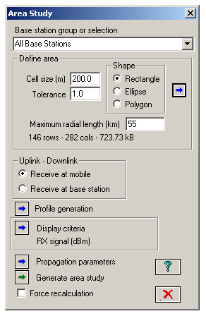
Area definition

The first step is to define the overall area, cell size and a tolerance for the calculation detail. Select the required shape and click the Shape button on the right side.

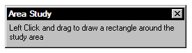
For a rectangular or elliptical shape:

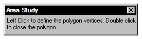
For a polygon shape:

Enter the Cell size and Tolerance to be used in the analysis. The overall dimensions of the study area and the cell size determines the number of rows and columns and the memory required for the area study data. If the area is too large or the cell size is too small, the memory allocation will fail and an error symbol will be shown in the dialog.

The area study generates a path profile from each base station to every cell in the defined area. On very large areas, this could result in path profiles several hundred kilometers long and which have no affect of the overall results. Provision has been made to limit the maximum profile length solely for the purposes of speeding up the calculation. If this field is blank, then the profiles will be generated to the maximum extents of the display.

Generate area study

Set the Display criteria and the Propagation parameters and click the Generate area study button to complete the analysis.

Carrier to interference calculation

The CtoI calculation starts with a downlink receive signal strength (RSS) calculation from each base station to each cell, as previously described. At this point, there will be an RSS value in each cell for every base station in the area study. In each cell the CtoI is calculated as follows:

• Determine the maximum RSS in the cell. Denote this signal as the carrier (C). All other RSS values in the cell become the interfering signals (I).
• The base station equipment setup dialog defines both the base station and the remote /mobile equipment parameters. If the study is for a mobile radio network, then the remote antenna would be omnidirectional and there would no antenna discrimination against interring signals. In this case, the remote antenna data file name is not entered and omnidirectional operation is used. If the study is carried out as a precursor to the design of a point to multipoint network, then an antenna file name should be entered for the remote antenna. This antenna pattern will be used to discriminate against the interfering signals. CtoI is the only display which uses the remote antenna pattern.
• Each base station sector can be assigned a channel number. This is actually done by assigning a color to each sector. The numbers in the color table become the channel number. If the corresponding frequency assignment is missing, then the CtoI analysis will be co-channel only. For example, a carrier on channel X can only be interfered with by another channel X. All other channel numbers will be ignored.
• If specific frequency assignments have been made for the base station sectors, then the additional loss due to the frequency difference can be calculated provided that both the victim remote radio and the interfering base station sector has been assigned a radio data file name. CtoI is the only display which uses the radio data files.
• Each interfering signal level is reduced by the antenna discrimination and frequency difference loss and the levels are added on a power basis. This addition is used for all duplex methods.

Carrier to interference calculation for different base stations types

Suppose the area study contains two different types of base stations one narrow band and the other wide band. The base stations operate in the same frequency band and the interaction between the two systems is to be analyzed.

The two types of base stations are placed in separate groups. Do not use a selection.

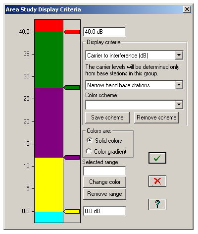
When the display criteria is set to Carrier to interference, an additional option is available to consider only one type of base station to determine the carrier level.

Suppose the Narrow band base stations group is selected. In each cell the maximum signal level will be determined from only signals in this group. All other signals will be considered interference.

The radio data files will require two sets of interference reduction factor curves:

One curve is required for interference from the same modulation - bandwidth and a second curve for interference from the other base station’s modulation - bandwidth.

Radio data interference curves

The following methods are used to calculate the loss due to the frequency difference between interfering signals and the receiver center frequency:

• Threshold to Interference (T- I) curves
• Interference reduction factor (IRF) curves
• Convoluting the interfering TX spectrum with the RX sensitivity curve. If the actual measurement data for these curves is not available, these will be created using masks based on the 3 dB bandwidth.

If T-I or IRF curves are not available, then the TX spectrum - RX convolution method is used which involves a numerical integration. Suppose the area display consisted of a 500 by 500 array with 5 base stations. Each cell would require 4 calculations resulting in 500 x 500 x 4 = 1,000,000 numerical integrations. This would result in an unacceptably long calculation time. To avoid this situation, create an IRF curve based on the channel bandwidth and the adjacent channel rejection. Assuming a channel bandwidth of 3.5 MHz, the points for the IRF curve would be as shown in the table below:

Simulcast delay spread

The simulcast delay calculation starts with a downlink receive signal strength (RSS) calculation from each base station to each cell as described above. The two strongest signals in a cell are analysed as follows:

• If the difference between these two signals is greater than the simulcast capture range specified for the mobile equipment, then no action is taken.
• In all other cases, the straight line distance time delay to each base station is calculated and the difference between the two values is used for the display criteria.

Most likely server

The receive signal strengths are calculated from each base station to each cell as described above. The most likely server color of the base station with the strongest signal is used for the display.

Empirical Studies

The propagation loss algorithms (TIREM, NSMA and Pathloss) are deterministic. That is, the calculations are made on the actual terrain profile. Empirical algorithms on the other hand are based on actual signal measurements for different conditions.

The following empirical algorithms are available for use in a local study scenario:

• F(50, 50), F(50, 10) and F(50, 90) curves
• Okumura (Hata)
• COST (Hata)

Right click on a site legend and select the Empirical studies menu item. A base station must be defined as is the case for local and area studies. Select the study method and enter or calculate the height above average terrain. The display criteria is used to specify the receive signal contour levels.

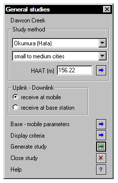
Click the Generate study button to display the signal contours.

Height Above Average Terrain (HAAT)

All of the empirical algorithms use the height above average terrain. A number of uniformly spaced radial profiles are constructed from the base station to a specified end distance. The average elevation for each profile is calculated from a specified start distance to the end of the profile. The average elevation of all profiles is then determined.

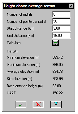
HAAT is the base antenna height above sea level minus the average elevation.

The default values for this calculation are shown on the right. All values are in metric units in the HAAT calculation.

 

F(50, 50), F(50, 10) and F(50, 90) Curves

The curves were digitized from the report:

Development of VHF and UHF propagation curves for TV and FM broadcasting - Report No. R-6602

Jack Damelin, William A. Daniel and George V. Waldo.

The display criteria is receive field strength expressed in dB mv /m and cannot changed.

The allowable frequency range for these curves are:

• 54 - 108 MHz - Channels 2 - 6 and FM
• 174 - 216 MHz - Channels 7-13
• 470 - 806 MHz - Channels 14 - 83

The terminology of the curves is as follows:

• F(50, 50) - 50% of the locations for 50% of the time
• F(50, 10) - 50% of the locations for 10% of the time
• F(50, 90) - 50% of the locations for 90% of the time

Okumura (Hata)

The basic path loss is given by:

(1)   

where:

f = frequency in MHz

hb = height above average terrain

d = path length

ahm = mobile height correction factor

 

For large cities:

(2)   

 

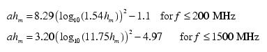
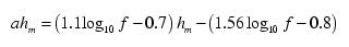
For small to medium cities:

(3)   

where hm = mobile antenna height above ground level in meters

For suburban areas, rural quasi open areas and rural open areas, a correction factor is applied to Lu using the small to medium cities definition for ahm given in Equation (3)

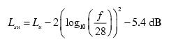
For suburban areas:

(4)   

 

For rural quasi open areas:

(5)   

 

For rural open areas:

(6)   

COST (Hata)

The COST (Hata) model is part of the COST 231 models which extend the frequency range of the Okumura (Hata) model described above.

The basic transmission loss is given by:

where:

cm = 0 for medium sized cities and suburban centers with moderate tree density

cm = 3 for metropolitan areas

f = frequency in MHz

hb = height above average terrain

d = path length in kilometers

ahm = mobile height correction factor

where:

h_m = mobile antenna height above ground level in meters.

For rural quasi open areas and rural open areas, the same correction factors as used in Okumura (Hata) are applied to the medium sized cities and suburban centers option.