What’s New in Pathloss 6

Pathloss 6 has taken on a number of major changes to how the program operates while maintaining a consistent and familiar interface. New program organization is aimed to simplify or eliminate many of the complexities involved in getting started or re-started with Pathloss. New design ideas are intended to allow Pathloss 6 to evolve and adapt to industry needs in the long term.

Program Organization and Layout

Pathloss 6 is installed as a single application. There is no separate application for links as there was in Pathloss 5. Pathloss 6 will show the network window, the link window or both depending on how it is being used.

Opening Pathloss 6 normally or by double clicking on a Network File (gr5) will bring up the network window as in Pathloss 5. From here you can open an existing network or begin adding sites and links in the usual way. Clicking on a link with the Link Tool will bring up the Link Window and open the associated file for that link.

You can click Files – New Link Window or click the associated toolbar button to bring up a new blank Link Window.

Unlike version 5, the Link Window is not restricted in its file operations. You can open a new link file, or click Files – New to start a new link. You can click Files – Add to Network at any time to move the working link in to the network.

Double clicking a link file (pl5, plz) on the desktop or in explorer will start a new instance of Pathloss and open the file directly in the Link Window. Pathloss will exit when this Link Window is closed. When operating in this mode you can click Files – Add to Network to bring up the link in the Network Window.

Link files can now be dragged and dropped on to the network window to add the link to the network. You can also import link files by clicking Files – Import Link File from the main menu. (Not in the Site List as in Version 5)

Tiled Map Backdrop

Pathloss now produces backdrop imagery for networks anywhere in the world.

Map tiles are downloaded and displayed automatically. Click and drag on the map to pan the display with any cursor and use the mouse wheel to zoom in and out. Map tiles are stored locally for efficiency and performance. You can enable\disable the automatic download of files by toggling Configure – GIS System – Network Display – Map Utilities – Download Automatically.

You can enable\disable the tiled map system entirely with Configure – GIS System – Network Display – Use Tiled Map Backdrop. If this option is disabled, Pathloss operates exactly as version 5, using projections and backdrops defined in the GIS Setup Dialog. At this time, the tiled map backdrop must be disabled to perform local or area studies. 

Backdrop Options

There are 3 map styles that can be switched between by using the menu Configure – GIS System – Network Display – Map Style… The options are Topographic, Street Map or Satellite. There will also be a method to allow the user to provide a custom tile provider of their choice.

By default, Pathloss starts with backdrop tiles enabled. To change the start up option, click Configure – Options – Program Options and select the Startup and Defaults section. The option is called Use Tiled Map Backdrop.

Backdrop Utilities

The map tile files are downloaded automatically and stored locally on the system. There are a few utilities for managing this data.

Occasionally a tile may not automatically download. In this case, right click on the missing tile and select Refresh Map Tile to re-download and display that tile.

There is a utility for deleting the cached map tiles.Click Configure – GIS System – Network Display – Map Utilities – Map Operations. Use the drop-down list to select whether to download files automatically or delete the locally cached tile.

Managed Terrain and Clutter Data

Pathloss 6 can automatically download and configure terrain data and clutter data from a number or sources. The following GIS data sets are currently supported in the managed system:

• SRTM 1" DSM (Global)
• ASTER 1" DTM (Global)
• NED 1" DTM (North America)
• NED 1/3" DTM (USA)
• Copernicus Global Land Cover 100m (Global)
• North American Land Cover 30m (NA)
• National Land Cover Database 30m (USA)

These data sources are used together to generate the terrain heights and define the type and heights of clutter on profiles. There is no need for a separate GIS configuration file if using the managed system. More sources will be added as they become available.

Please see the following topic for more information and usage Terrain Data and GIS Configuration

Manual DEM and Clutter Setup

One or both of the managed terrain and clutter models can be set to Manual DEM / Clutter Setup. This allows the user to use the GIS Setup dialog to define and import custom GIS data (such as Lidar or local formats) in to Pathloss 6. Click Configure – GIS System – GIS Setup Dialog to open the dialog. The operation of the dialog is similar to version 5. The GIS file is saved with extension p6g. The Version 6 GIS File stores the managed Terrain and Clutter model selections as well as the Tiled Backdrop usage and will apply them when loaded. Version 5 p5g files can also be loaded directly from the GIS Setup dialog.

Terrain Data

The GDAL (gdal.org) library is now integrated in to the Pathloss Vector and DEM systems. This allows direct support of many sources globaly with out conversion.  

GeoTIFF Raster DEM and Clutter File Support

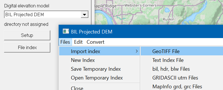
Pathloss 6 can now index and use GeoTIFF format files in the Primary and Secondary DEM indexes. This will allow Pathloss 6 to use data from many sources that use GeoTIFF such as ASTER, CDEM, etc. To use GeoTIFF files, select the BIL Projected DEM or BIL Geographic DEM option as the Digital Elevation Model. Then click File Index to open the Index window. Select the Menu Item Import - GeoTIFF File. You can select one or multiple GeoTIFF files for import.

Pathloss will automatically set the projection from information encoded the first GeoTIFF file. If Pathloss is not able to determine the projection, the parameter string will be displayed to the user so the projection might be set manually.

GeoTIFF Files can also be used in the Clutter index by selecting BIL Projected Clutter or BIL Geographic Clutter and using the same menu item. GeoTIFF Files can be used for either height or category style clutter. In the case of category clutter, the definition table must be filled out manually for now. 

GeoJSON Vector Formats and Tiled Vector Building Data

Support for GeoJSON (.json) format vector files has been added to the vector system. These vectors can be added to the vector index by the usual method: Files - Import - Vector Files.

Tiled Vector Building Data Support

Building data is often distributed as vector tiles arranged in a folder tree. In this case, rather than adding the individual files, the entire folder structure can be added as a single vector entity. Click Files - Import - Vector Tile Folder. Select the top level folder of the tiled data. Double click on the Building Height Field and select the correct entry for your data-set. You can also change the color and attributes of the data-set from the Definition Table.

The data is now ready to use. In addition, any new files added to the folder structure will automatically be processed the next time that network or GIS file is loaded.

Vector Building Data can be obtained from a number of sources both free and commercial such as:

https://3dbuildings.com/

Multiband

PLZ File Format

Pathloss 6 is utilizes an extensible file format for storing all information necessary for link design. This file has the extension plz and is currently used for multiband and passive repeater links. links.In the future, this format can be used to bundle radio and antenna equipment data with the link, store a complete passive design, and handle any future data requirements.

Multiband operation allows you to add an additional set of equipment to an existing link. Each band will contain a complete set of equipment parameters, antenna heights, a channel table, design frequency and polarization. The site information, path profile and all calculation options are common to all bands in the link.

Creating a Multiband Link

Open a link or bring up a new link window with Files – New Link Window.

You can add a new band to the link by clicking Operations – Multiband – Add Band – Copy Current Band. This will create a new band that is a duplicate of the first. The title bar of the link window shows the current band and total number of bands (Pathloss switches to the new band when it is added.)

Note when you add a second band to a link, the link filename will change to .plz  The original link file (pl6), if any, is not modified. When you next save, if the link is in the current network, you will be prompted to update the network file association with the new .plz filename.

You can now edit the band information manually or by other methods such as a link design rules file or by loading an existing link file as a template. Any changes to the equipment, antenna heights, frequency, channel table, or polarization will apply only to the current band. Any changes to the profile, or calculation options will apply to the link as a whole. This is true whether the changes are made manually or by using the auto designer or other methods. In the future, design of the band may be performed automatically as it is added.

To select a different band, use the menu Operations – Multiband – Switch Band… Or you can move to the next band by pressing Ctrl + B. To remove the current band, click Operations – Multiband – Remove Band.

Integration of multiband and the plz format in general is an ongoing process. Currently, plz files can be imported in to and opened from a network, but will not operate with batch network operations or reports. The interference operation has initial support for multiband links and is currently being tested.

Carrier Aggregation

The Carrier Aggregation report works with multiband links to determine the sum capacity of the link over the range of availabilities. This is a purely mathematical operation and by its nature assumes that the multipath fade probabilities in each band are independent from one another i.e., best case.

Carrier aggregation depends on the radio file having capacities defined for each modulation state. These should be in the file as a number in Mbps.

Multipath Aggregation Algorithm

Each band contributes a certain capacity for some percentage time of the year – Availability or “Time in Mode”. The algorithm determines all possible combinations of these states between bands. For each combination, the sum of the capacity and the probability of this combination occurring is computed.

As an example, we can look at a dual band configuration where each band is a fixed modulation. Therefore, each band is either available or unavailable. There are 4 possible combinations: both available, one or the other available, or neither available.

If we look at the same dual band configuration except now each band has 3 modulation states. Each band can then contribute 4 possible capacities after accounting for no capacity when the band is unavailable. Therefore, there are 4x4 = 16 possible state combinations.

The total capacity of a combination is the sum of the state capacities. Combination State Time is defined as the percentage of the year this combination is expected to occur and is calculated as the product of the “time in mode” values for each state. The availability of a state combination is defined as the availability of that capacity or greater.

Rain Consideration

For each state in a multiband system, a critical rain rate is determined. As the rain rate increases, any bands with a critical rain rate at or below that level will no longer contribute capacity. This rain calculation determines what combinations will be in effect at the critical rain rates and estimates the occurrence of those rates over the year.

The rain outage probabilities are also combined with the multipath values in the combinations above to produce a total availability for each combination and a reduced Combination Time.

Carrier Aggregation Report

Click Operations – Multipath – Carrier Aggregation Report to perform the calculation and view the results.  The dialog box has three areas: the control panel on top, a plot display of capacity across the domain of availabilities, and an information panel below that.

The plot display shows the aggregate capacities between a minimum and maximum availability. You can use the mouse wheel with the cursor over the plot display to adjust the minimum availability. Hold Ctrl and use the mouse wheel to adjust the maximum availability. Hold Shift plus mouse wheel to “scroll” the display by adjusting both availability bounds. Left click to select a state for detailed display. You can also set the minimum and maximum availability by typing the value in to the controls on the left.

The information panel can show a summary of the multiband calculation, detailed information about a particular combination, or the effect of rain. You can use the radio buttons at the bottom of the controls to select what is displayed. You can also click on one of the bars in the plot display to show the details for that combination.

Settings

You can change the calculation options in the top part of the control panel. These settings affect how the results are presented:

• Group Low occurrence combinations. This option will groups relatively uncommon combinations with the next lower 'common' combination. Each combination that occurs for less that 5% of the time of the next lower common combination will be grouped. You can view the detailed display for a state to see all combinations that are contributing ordered by expected amount of time.
• List all combinations in report. If this option is unchecked, only the most commonly occurring combination will be shown in the report. Otherwise all the grouped combinations will be listed ordered by occurrence time. 
• Output CSV will print the capacity vs. availability data at the end of the report as a simple csv.

Click Save and Close to accept the settings. These will be stored with the plz file when it is next saved. Or click Save and Show Report to save and close the dialog and generate the report in the RTF report window. Cancel closes the dialog without saving.

Unlimited Number of Channels in Link Files

New TX Channel Interface

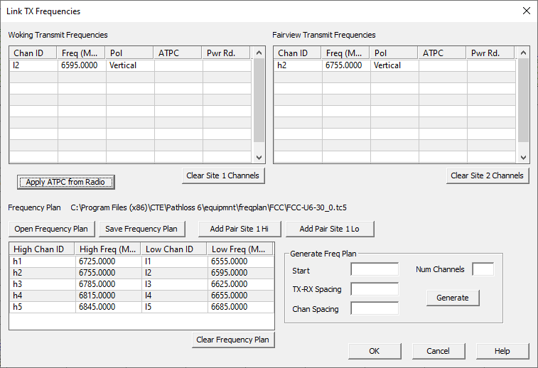
A new interface was developed in order to manage the increased number of channels. The frequency plan is also integrated in to the dialog for easy access and to encourage use. There are three grids for entering data: one TX Channel List for each end of the link, and a Frequency Plan. The grid interface works similar to other grid controls (SiteList), in Pathloss including all expected keyboard operations. When working in a grid control, pressing Escape once will cancel any open cell edit. Pressing Escape again will set the focus back to the dialog so that the keyboard can be used to close the dialog by pressing Enter or Escape. Closing by pressing Enter will keep changes and pressing Escape will prompt to save if needed.

Data can be entered on any row but will be consolidated when closing the dialog. Only channels with a valid frequency are retained. There are an unlimited number of rows, press the down arrow key on the last row to add more rows.

The Frequency Plan is shown at the bottom of the dialog, along with controls to Open or Save frequency plan files (.tc5). Channel pairs can be added to the link by highlighting the row in the frequency plan and pressing one of the two Add Pair buttons (Site 1 Hi or Site 1 Low). There is also a section to generate a frequency plan by entering a channel spacing, a tx-rx spacing, and a starting frequency.

There is a field to enter an id format string. In this string, use "%d" to output the channel number or "%0Nd" to pad with zeros to make the output N characters wide. The ID is the appended with an 'H' or 'L'.  For example, if the format string was "Chan-%03d", the first id pair would be Chan-001H and Chan-001L.

This interface is used when clicking the Site 1 or Site 2 Channels button in the Transmission Analysis module. It is also used in the Assign Frequencies operation and the Site Interference operation.

Industry Standards

In addition to all of the standards in Pathloss 5, Pathloss 6 adds support for the following ITU standards

ITU-R P.530-18 - Propagation data and prediction methods required for the design of terrestrial line-of-sight systems

ITU-R P.530-17 - Propagation data and prediction methods required for the design of terrestrial line-of-sight systems

ITU-R P.837-7 - Characteristics of precipitation for propagation modelling

ITU-R P.676-12 - Attenuation by atmospheric gases and related effects

ITU-R P.835-6 - Reference standard atmospheres

ITU-R P.453-14 - The radio refractive index: its formula and refractivity data

ITU-R P.530 XPD calculation option. 

Pathloss 6 also adheres to the standards set out in the TIA (Telecommunications Industry Association) Standard TIA-10 Interference Criterion for Microwave Systems.

Also in Pathloss 6 is an experimental version of the Vigants-Barnett Multipath Fading algorithm that takes in to account path inclination.  

FCC ULS Integration

Pathloss 6 includes support for the FCC ULS Database system. Users working in North America can download the FCC’s ULS data and use it in Pathloss to perform interference calculations against Pathloss designs. This feature is only available with the Interference option.

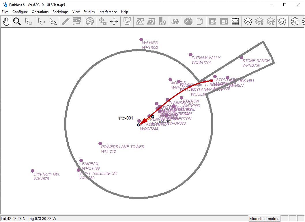
Licenses requiring coordination are displayed graphically in the new Browse Interference cases window. The NSMA defined coordination area is displayed along with the stations that met the interference objective. The user can toggle though the cases and sub cases and the interfering path is displayed. Users can click on an interfering site, and the site details are displayed. This initial release displays the following information:

• Site name
• Callsign
• Owner details and contact information
• All coordinating stations for the license

The download process is fast and simple using the dedicated ULS Data Download (UDD) program. New License data is published every Sunday on the FCC website.

 

 

 

Installation and Licensing

Pathloss 6 is now installed a single program with no standalone link program. This reduces complexity and enhances the relationship between the link and network window. The standalone utility AntRad is also included as part of the standard installation.

Pathloss 6 is compliant with modern Window application hierarchy which allows a wider range of installation environments and licensing options. Window 11 is fully supported.

The Pathloss 6 graphics system has been updated to work with 4K monitors and greatly improves rendering performance.

Google Earth Export

The network Google Earth export now uses .kmz format so that it can be used and transferred as a single unit. There is also the option to export the link Fresnel zones to google earth as well. There is a new toolbar button associated with the Google Earth export. In the future this button will open the network in google earth without needing to save a kmz file first.

Roadmap

Pathloss 6 will be evolving continuously and take on considerable improvements in the near term, both pre and post release. Some of the important planned features are summarized below.

Local and Area Study Rework

Local and area studies will be reworked to bring them inline with modern LTE design requirements. These changes will generalize the system and allow it to display on the tiled map display and utilize more building\cutter data types. Changes will be made to the internal base station layout so that sector definitions are more intuitive and flexible. More options for defining the area of the study and the ability to export the raw data in csv format will also be included. This will be completed before the official release.

PLZ, Multiband Integration and Network Operations

The use of the plz format will be expanded upon to allow simplified handling of passive links or for bundling equipment files in with the link. The plz format will be integrated in to the network operations and design system. Likewise, multiband files will be integrated in to existing systems such as interference calculations, automated design and reports. This will be completed before the official release. For the time being, the transmission analysis window is the only place plz files can be created.

NLOS Experimental Work

This build includes some temporary experimental options to allow customization of the tree loss component in the diffraction module. For the time being, there are 2 simple options for modifying tree loss effects: Effective Tree Height, which scales the height of any vegetation clutter, and Overall Weight Factor, which simply diminishes the final tree loss. These are currently only intended for testing. As we continue to examine the algorithm and results from field tests, we hope to establish some simple tools to customize the tree loss calculation to particular climates or databases.

Reports

We are currently examining options for a replacement to the existing customizable report system.

Pathloss 6 Development Roadmap

Pathloss 6 is under continuous development. Features and improved functionality are added during it's life cycle. A roadmap of this development can be found here: Pathloss 6 Development Roadmap