Geographic Information System (GIS) Configuration
Overview
Pathloss 6 has many new features for managing terrain data automatically, but there may be cases where users are working with terrain data outside of the automatic sources. The scope of this help section is to guide the user in setting up a manual GIS Configuration.
Some data sources are no longer available but have been included in the documentation for users wanting to work with these legacy datasets. These datasets are labeled LEGACY, and the user should consider using more current higher resolution datasets.
Select the Configure-Set System-GIS Setup Dialog from the menu. This dialog defines the following components of the Pathloss program’s geographic information settings:
- Site coordinates
- Digital elevation models (DEM) for terrain profile generation and elevation backdrops
- Terrain clutter database to add clutter to terrain profiles and for clutter backdrops
- Backdrop imagery - (Ortho photos, Scanned imagery, Maps)
- Vector data
The setup procedure is organized in seven tabs.
GIS files (*.P6G)
The GIS settings are saved in a file with the suffix *.p6g. These files are not automatically saved. Click the GIS files button to access the files menu. The file name should reflect the geographic area and possibly the specific data formats used in the file.
The network display file (gr5 file) includes the full path name of the p6g file. When the network display file is loaded, the associated p6g file will be automatically loaded.
Datum and Projection Definition
Each of the tabs in the GIS setup include a datum and projection definition. Some of these will be automatically set by the program. For example, when an SRTM digital elevation model is selected, the datum is set to WGS84 and the projection to geographic. In other cases, the user must set these parameters; and therefore, an understanding of these terms is necessary. The following paragraphs provide a brief description of these terms as they are used in the Pathloss program.
Datum
A datum is a horizontal reference used to specify latitude and longitude coordinates. The same coordinates in different datums will point to different locations. Conversely, the same location in different datums will have different coordinates. Basically there are two types of datums: local or geodetic and geocentric. The reference point for geocentric datums is the mass center of the earth. The reference point for a local datum will be some monument in the area. For example, the reference point for the North American datum of 1927 (NAD27) is a triangulation station at Meades Ranch in Kansas.
The errors between coordinates expressed in different geocentric datums (e.g NAD83 and WGS84) are not significant; however, serious positional errors can occur if the coordinates belonging to a local datum are used in a geocentric datum or vice versa. Several examples of these errors are given in the table below.
| Local Datum | Geocentric Datum | Latitude | Longitude | Error (m) |
| NAD 1927 | NAD 1983 | 65 North | 145 West | 120 |
| NAD 1927 | NAD 1983 | 56 North | 120 West | 89 |
| NAD 1927 | NAD 1983 | 35 North | 115 West | 74 |
| NAD 1927 | NAD 1983 | 26 North | 82 West | 45 |
| ED 1950 | WGS 1984 | 42 North | 12 East | 131 |
| OS 1936 | WGS 1984 | 52 North | 0 | 121 |
| AGD 1966 | GDA 1994 | 35 South | 145 East | 204 |
| AGD 1966 | GDA 1994 | 25 South | 115 East | 198 |
The datum definition contains the following information:
- Major and minor axis of the earth. These are used in the great circle arc distance calculations.
- Parameters to transform coordinates between this datum and the WGS 1984 datum. In order to improve the transformation accuracy, the overall area of the datum may be divided up into smaller regions. Each region has its own transformation parameters. Therefore, in the case of local datums, the user needs to specify the specific region for the datum.
Projection
A projection converts coordinates between spherical (geographic latitude and longitude) values and rectangular x, y values. The rectangular format is required to display geographic information on a flat surface. In the Pathloss program, the projection category “Geographic” means latitude and longitude. In other words there are no rectangular x, y values.
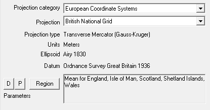 The projections are loosely organized alphabetically. Many projections such as the British National Grid or the Swiss National System are unique and when one of these categories are selected, the corresponding datum will be automatically set. If the datum contains multiple regions, the user must set the region. On other projections, such as the Universal Transverse Mercator projection, the user must explicitly set the datum.
The D and P buttons show the specific datum and projection parameters.
Fixed and variable zone projections
To control the distortion inherent in a rectangular projection, limits are set on the valid area of projection. For the Transverse Mercator projection, the east - west limits are in the order of 6 degrees of longitude and the overall area is divided up into zones. Several special cases of this projection are:
- Universal transverse Mercator (UTM) - Zone 1 to 60 in 6 degree increments
- Australian map grid (AGD66, AGD84 and MGA94) - Zone 47 to 58 in 6 degree increments
- Gauss conform South Africa - Standard Meridians 17 to 31 degrees east in 2 degree increments
In these cases, the user can choose to specify the zone (fixed zone) or have the program calculate the zone based on the longitude (variable zone).
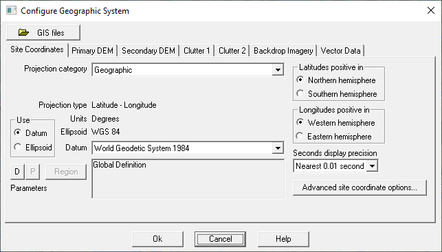
Site Coordinates
In the Site coordinates tab, set the datum corresponding to your site coordinates. Site coordinates are always expressed in latitude and longitude. If a projection other than geographic is specified, then both coordinate formats are available. Data can be entered in either format and the other format will be automatically calculated.
In most cases, the geographic setting is recommended. If a UTM projection is required, the variable zone is recommended. A projection must be set for the following conditions:
- Site coordinates are only available in a projected format.
- Site data is being imported from a text file. The coordinates in the text file are in a projected format. In this case, the site coordinates projection must be set to the same projection used in the text file. Once the import is complete, the projection can be changed back to geographic.
Note that the datum and projection settings here only applies to the site coordinates. The terrain database, backdrop imagery and vector data may have different datums and projections.
Latitude - Longitude Sign Convention
By convention, latitudes are positive in the northern hemisphere and negative in the southern hemisphere. Longitudes are positive in the eastern hemisphere and negative in the western hemisphere. For manual data entry, an option is available to enter latitudes and longitudes as positive numbers. The coordinates are formatted using the letters N/S and E/W for latitudes and longitudes respectively. This is a good indicator that the correct sign was used. Refer to the Data Entry section for details on the data entry format for coordinates.
Seconds Display Precision
The coordinate format can be set to the nearest second( 56 08 28 N), the nearest 0.1 second (56 08 28.4 N) or the nearest 0.01 second (56 08 28.43 N). This is for reporting purposes only and does not affect the precision. Coordinates are stored as double precision numbers in the program.
Advanced Site Coordinate Options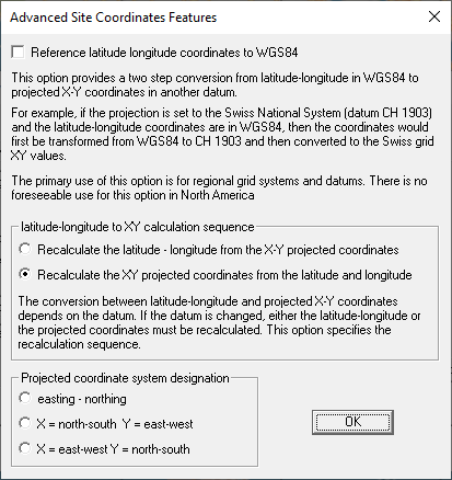
Reference latitude and longitude coordinates to WGS84
The situation arises when projected coordinates are used exclusively, and latitude and longitude are not available. Suppose the site coordinates are setup to use the British National Grid projection. The corresponding datum is the Ordnance Survey Great Britain 1936 and the region is set to England.
The initial grid coordinates are X = 540000, Y = 235000 meters. The corresponding latitude and longitude are 51 59 43.25N and 00 02 21.85E. Note that these coordinates are referenced to the OSGB36 datum.
Suppose now that these coordinates were inadvertently used assuming a WGS84 datum. The error would be 113.6 meters in X and 47.7 meters in Y.
If the Reference latitude and longitude coordinates to WGS84 option is checked, then a two step conversion is used from latitude-longitude (WGS84) to British National Grid X-Y. The intermediate latitude and longitude in OSGB36 are not displayed. In effect, this option allows GPS coordinates in WGS84 to be used directly.
Latitude Longitude - to Grid Coordinate Calculation Sequence.
If the user enters the latitude and longitude, the projected grid coordinates are calculated and vice versa. Note that this calculation depends on the datum (major and minor axis of the ellipsoid).
Suppose the user has taken the UTM eastings and northings for a series of sites from a topographic map and entered these into the program. The user then notices that the datum was incorrectly set; and therefore, the latitude and longitude values are wrong. To salvage the work, the user would set the calculation sequence to Recalculate the latitude - longitude from the projected XY coordinates and then change the datum.
Projected Coordinate System Designation
This option specifies the grid coordinate labels in data entry forms and reports. The easting and northing designations are unambiguous; however, X and Y designations can have opposite meanings on some projections. For example, in the Swiss National Grid system, X corresponds to northing and Y to easting.
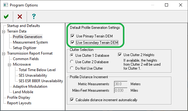
Primary and Secondary DEMS
A Primary and Secondary DEM can be configured. Their usage is controlled by the profile generation options under the menu item Configure - Program Options -Terrain Data - Profile Generation. If both primary and secondary databases have been configured and are checked in the options, the program will start with the primary database. If the operation (profile or elevation backdrop) is not complete, then the secondary database will be used to fill in the missing sections. Therefore, the primary database should have the best resolution.
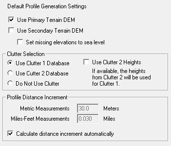 The default and recommended setting is to use the primary DEM only. If the operation fails then it is a simple matter to enable the secondary DEM and the user can inspect the different areas in which this DEM was used.
When a profile is generated for the first time, the DEM file usage is written to the notepad.
Note that it is possible to configure a DEM with different data sources provided that they are both in the same database category and are referenced to the same datum. For example, in the BIL geographic database, one could load the GTOPO30.ndx index file and then add SRTM files to the index. When two files cover the same area, the program will use the file with the best resolution.
The Pathloss program does not have a proprietary DEM format. Instead, the program uses the various industry standard formats directly. Some DEMs are only available in an ASCII format. In these cases, the ASCII files must first be converted to a binary format.
The following sections provide the setup procedures for the various database formats supported by the program.
On completion of the setup procedure, generate a path profile in the Terrain Data module. The site coordinates must be within the south-north and west-east edges of the DEM file. In the case of the generic BIL databases, some of the default DEM parameters may need to be changed based on the results of this test profile. In the primary or secondary DEM tab, click the File index button and then select the Edit - Parameters menu item or right click on a data cell.
- Byte order - Change from Motorola-Spark to Intel or vice versa if the elevations are missing or erratic.
- File origin - Change the origin from the SW corner to the NW corner or vice versa if the elevation backdrop appears to be upside down.
- Treat no data values as sea level - Use this setting if elevations are missing when a portion of the profile is over water. The missing values will be replaced by 0 elevations.
SRTM Setup Procedure
SRTM Data is now part of the Automatic Terrain Management system in Pathloss 6. The instructions below can be used for previous versions of the Pathloss program.
SRTM (Shuttle Radar Topography Mission) data is probably the most widely used terrain data at present. The data is available in a 1 arc second resolution from 60 degrees south to 60 degrees north worldwide. By nature of the data acquisition technique, the elevations include buildings and tree cover to a certain extent; and therefore, this database can be considered as a quasi composite elevation - clutter database.
This setup procedure will use hgt files. The first step will be to determine the names of the required files. The file names are 7 characters long and are based on the latitude and longitude of the south west corner of the one degree square block which surrounds the data point. The table below gives several examples in the various hemispheres.
| Latitude | Longitude | hgt file name |
| 45 23 14.26N | 96 34 12.34W | N45W097.hgt |
| 45 23 14.26N | 96 34 12.34E | N45E096.hgt |
| 45 23 14.26S | 96 34 12.34W | S46W097.hgt |
| 45 23 14.26S | 96 34 12.34E | S46E096.hgt |
In the network display, the required SRTM file names for a link can be found as follows:
- Select the Configure-GIS System-GIS Setup Dialog from the menu and verify that the site coordinates projection is set to geographic.
- Select the Configure - Options - Network Display Options - Axis - Map grid menu item. Set the Map names to SRTM - Aster grid and then check the Show geographic grid and Show labels on grid options.
- Right click on a link and select the Map crossings menu item.
- A report will be created which shows the required STRM files for that link.
SRTM data files are downloaded directly from CTE using the FetchSRTM program. The files will be received in a zipped format. Create a directory for these files and unzip the files into this directory.
- Select the Configure-GIS System-GIS Setup Dialog from the menu and then select the Primary DEM tab.
- In the Digital elevation model drop-down list, select STRM (world). This DEM is a preconfigured type using the BIL geographic base type. The projection is automatically set to Geographic and the datum to WGS84. Do not change these settings.
- The next step is to specify the location of the hgt files. If all file are in the same directory, click the Setup button and select the directory; however, it is often expedient to assign the directories as part of the file indexing step described next.
- Click the File index button and then select the Files - Import index - SRTM hgt files menu item.The SRTM file selection dialog appears which includes a File directories selection. The default is always Use individual file directories. This is a multiselect file selection dialog. Hold down the shift or ctrl key to multiselect the hgt files and click the Open. button The file index will be created using the file name. The resolution 3 seconds or 1 second is determined by the file size.
- Close the File index and save the p5g file. This completes the setup procedure for the SRTM terrain database
Note that there is considerable overlap in the Import index menu above. The first selection bil, hdr, blw files is intended for SRTM files in the BIL data format. Other database types can be used in the same index provided that they use the same datum and projection. If the index contains several different resolutions, the entire index will be read to ensure that the file with smallest cell size is used.
Bad or missing data in SRTM files
Many SRTM files contain bad or missing data. The nodata value used in SRTM files is -9999. This is usually the result of incomplete data collection for the file; however, sometimes this nodata value is used for sea level areas. Advanced users may consider setting the option Treat nodata values as sea level; however, this is not a good plan as entire islands can be missed with this approach. This option is available in the File index under the Edit - Parameters menu item.
On completion of a SRTM setup or modification, always generate an elevation backdrop and look for missing data. The default no data color is set under the Backdrops - Elevation color ramp menu item. In the Terrain data module, a path profile will show any nodata values encountered in the files and these can be corrected manually. In any of the automated design operations, any bad or missing data will stop the design operation on that link. In local and area studies, the profile generation will continue to the end of the profile. If missing data was encountered, then only the profile up to the first nodata value will be used in the analysis and the final display will show gaps starting at these points.
In most cases, the missing data is scattered in very small areas sometimes on a single point. In these cases, a reasonable solution would be to use the secondary DEM to fill in the missing data. GTOPO30 represents a fair compromise for these small areas.
NED GridFloat Setup Procedure
The previous section described the setup procedure for NED_INT16 data. It was noted that this data is also available in a GridFloat format. This section describes the procedure for the GridFloat data. Data in this format is usually supplied on an external hard disk.
Each directory contains several files including a header file (hdr), projection file (prj) and a world file (blw). These are required to create the NED file index. The elevation data is contained in the bil file.
- Select the Configure-Set System-GIS Setup Dialog from the menu and then select the Primary DEM tab.
- In the Digital elevation model drop-down list, select GridFloat (NAD83). This DEM is a preconfigured type using the BIL geographic base type. The projection is automatically set to geographic and the datum to the North American Datum of 1983. Set the specific region as required. Do not change these settings.
- The Setup button is used to set the directory when all files are in the same directory. The GridFloat files will be in different directories and this step is not required.
- Click the File index button and then select the Files - Import index menu item.
- To create an index for a single download directory, select the Create from hdr-prj files menu item. The Gridfloat file selection dialog appears which includes a File directories selection.The default is always Use individual file directories. Go to the directory and select the gridfloat file to create the index
- To create an index for multiple directories, select the Create for folders - subfolders menu item. Select the top level directory.
- Older gridfloat files did not use a file suffix. At present gridfloat files use the suffix grd. Set the Files of type to gridfloat - new.
- The index will be created for this directory and all directories below this one. The directory structure should contain only gridfloat elevation files.
- Close the File index and save the p5g file. This completes the setup procedure for the GridFloat terrain database.
GTOPO30/SRTM30 Setup Procedure
GTOPO30/SRTM30 is a global dataset covering the full extent of latitude from 90 degrees south to 90 degrees north, and the full extent of longitude from 180 degrees west to 180 degrees east.
The most common use for GTOPO30/SRTM30 in Pathloss is for filling in overwater gaps on profiles where files don't exist for areas that are water only with no land mass. For this reason users should set up GTOPO30/SRTM30 as the Secondary DEM.
The SRTM30 files can be downloaded at:
https://pathloss.com/pwiki/index.php?title=SRTM30
Setup Procedure
- Select the Configure-GIS System-GIS Setup Dialog and then select the Secondary DEM tab.
- In the Digital Elevation Model drop-down list, select GTOPO30 (World). The projection is automatically set to Geographic and the datum to WGS84. Do not change these settings.
- Click the File index button and note that index is predefined, and; therefore, only the DEM files are required (*.dem).
- Click the Setup button and set the main directory for the GTOPO30 files. This completes the setup procedure for the GTOPO30 data.
Usage
In the Program Options or the Generate Path Profile window, Check the Use Secondary DEM along with the Use Primary DEM checkboxes.
During profile generation, when the program encounters a missing file in the Primary DEM, it will use the Secondary DEM.
More information
GTOPO30/SRTM30 have the following characteristics:
- The elevations are organized in rows running from west to east starting at the north west corner.
- The elevations are 2 byte integers in the Motorola (big-endian) format.
- The spatial reference is geographic with a resolution of 30 arc seconds.
- The datum is WGS84.
The elevation values range from -407 to 8,752 meters. In the DEM, ocean areas have been masked as "no data" and have been assigned a value of -9999. Lowland coastal areas have an elevation of at least 1 meter, so if a user reassigns the ocean value from -9999 to 0 the land boundary portrayal will be maintained. Due to the nature of the raster structure of the DEM, small islands in the ocean less than approximately 1 square kilometer will not be represented. The complete GTOPO30/SRTM30 file set is shown in the following table:
Note that the resolution of this data-set is 30 arc seconds. This means that the cell size is approximately 921 meters by 921 meters at the equator. The elevations represent the average values in the cell. At higher latitudes the cell width will decrease; however the overall resolution is inadequate for any detailed design. The GTOPO30/SRTM30 dataset is useful for backdrops and for diagnosing setup problems with other data sets.
| File name | Latitude | Latitude | Longitude | Longitude | Elevation | Elevation |
| W180N90.DEM | 40 | 90 | -180 | -140 | 1 | 6098 |
| W140N90.DEM | 40 | 90 | -140 | -100 | 1 | 4635 |
| W100N90.DEM | 40 | 90 | -100 | -60 | 1 | 2416 |
| W060N90.DEM | 40 | 90 | -60 | -20 | 1 | 3940 |
| W020N90.DEM | 40 | 90 | -20 | 20 | -30 | 4536 |
| E020N90.DEM | 40 | 90 | 20 | 60 | -137 | 5483 |
| E060N90.DEM | 40 | 90 | 60 | 100 | -152 | 7169 |
| E100N90.DEM | 40 | 90 | 100 | 140 | 1 | 3877 |
| E140N90.DEM | 40 | 90 | 140 | 180 | 1 | 4588 |
| W180N40.DEM | -10 | 40 | -180 | -140 | 1 | 4148 |
| W140N40.DEM | -10 | 40 | -140 | -100 | -79 | 4328 |
| W100N40.DEM | -10 | 40 | -100 | -60 | 1 | 6710 |
| W060N40.DEM | -10 | 40 | -60 | -20 | 1 | 2843 |
| W020N40.DEM | -10 | 40 | -20 | 20 | -103 | 4059 |
| E020N40.DEM | -10 | 40 | 20 | 60 | -407 | 5825 |
| E060N40.DEM | -10 | 40 | 60 | 100 | 1 | 8752 |
| E100N40.DEM | -10 | 40 | 100 | 140 | -40 | 7213 |
| E140N40.DEM | -10 | 40 | 140 | 180 | 1 | 4628 |
| W180S10.DEM | -60 | -10 | -180 | -140 | 1 | 2732 |
| W140S10.DEM | -60 | -10 | -140 | -100 | 1 | 910 |
| W100S10.DEM | -60 | -10 | -100 | -60 | 1 | 6795 |
| W060S10.DEM | -60 | -10 | -60 | -20 | 1 | 2863 |
| W020S10.DEM | -60 | -10 | -20 | 20 | 1 | 2590 |
| E020S10.DEM | -60 | -10 | 20 | 60 | 1 | 3484 |
| E060S10.DEM | -60 | -10 | 60 | 100 | 1 | 2687 |
| E100S10.DEM | -60 | -10 | 100 | 140 | 1 | 1499 |
| E140S10.DEM | -60 | -10 | 140 | 180 | 1 | 3405 |
| W180S60.DEM | -90 | -60 | -180 | -120 | 1 | 4009 |
| W120S60.DEM | -90 | -60 | -120 | -60 | 1 | 4743 |
| W060S60.DEM | -90 | -60 | -60 | 0 | 1 | 2916 |
| W000S60.DEM | -90 | -60 | 0 | 60 | 1 | 3839 |
| E060S60.DEM | -90 | -60 | 60 | 120 | 1 | 4039 |
| E120S60.DEM | -90 | -60 | 120 | 180 | 1 | 4363 |
| ANTARCPS | -90 | -60 | -180 | 180 | 1 | 4748 |
DTED Setup Procedure
DTED (Digital Terrain Elevation Data) is the US Defense Mapping Agency binary terrain data format. The basic DTED data format is given below:
- The elevations are 2 byte integers in the Motorola (big-endian) format.
- The elevations are organized in columns running from south to north starting in the south west corner. Each column begins with a header and ends with a check sum of the elevations.
- The elevations are defined at the intersection of the row - column grid lines.
- The datum is WGS84.
- The spacial reference is geographic (latitude - longitude).
- The east - west resolution is 3 arc seconds for DTED level 1 and 1 arc second for DTED level 2. The north - south resolution varies with latitude as shown below for DTED level 1 data:
- 0 to 50° - 3 sec
- 50° to 70° - 6 sec
- 70° to 75° - 9 sec
- 75° to 80° - 12 sec
- 80° to 90° 18 sec
Select the Configure-Set GIS configuration and then select the Primary or Secondary DEM tab
In the Digital elevation model drop-down list, select DTED. The projection is automatically set to Geographic and the datum to WGS84. Do not change these settings.
Click the Setup button. DTED files can be configured to use a file naming convention or a file index. If only a small number of files are available, use the file index method. The two methods are described below.
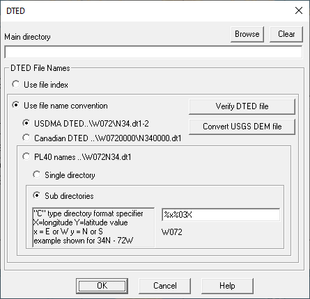
File Index
If all files are in the same directory, click the Browse button and set the directory; however, it is often more expedient to assign the directories as part of the file indexing step.
Check the Use file index option and then click the OK button to close the Setup dialog. No further settings are necessary for this method.
Click the File index button and select the Files-File index menu item. Multiselect the DTED files and click the Open button to create the index.
Note that the index can contain both level 1 and level 2 files (dt1 and dt2). In areas covered by files with both resolutions, the highest resolution file will be used.
File naming convention
Several file naming conventions and directory structures are available for DTED files. The file suffixes for level 1 and level 2 data are dt1 and dt2, respectively. In all cases the Main directory must be set. Click the Browse button and set this directory.
- USDMA defined directory names are based on the longitude e.g W072. File names in that directory are based on the latitude e.g. N34.dt1. In this arrangement the full path file name would be (main directory)\W072\N34.dt1.
- Canadian DTED file naming convention - this is the same as the USDMA convention with four zeros added to the directory and file names. The full path file name in this case would be (main directory)\W0720000\N340000.dt1.
- The Pathloss version 4.0 file naming convention uses the latitude and longitude e.g. W072N34.dt1. The file name is unique and does not depend on the directory name. The files can be all located in a single directory or can be saved in a user defined data structure based on latitude or longitude. Using the directory format specifier “%x%03X”, the full path file name would be (main directory)/W072/W072N34.dt1
USGS ASCII to DTED file conversion
USGS 1:250,000 ASCII DEM files can be converted to the DTED file format.
In the Setup dialog, click the Convert USGS DEM file button. Multiselect the USGS ASCII files and click the Open button to convert the files.
In the File index. select the Convert - USGS DEM menu item. Multiselect the USGS ASCII files and click the Open button to convert the files. The conversion will automatically create an index.
Verify
Each column of data in a DTED file includes a check sum of the elevations in that column. To verify the data integrity using this check sum:
In the Setup dialog, click the Verify DTED file CRC button when using the file naming convention. Multiselect the DTED files to verify and click the Open button.
In the File index, place the cursor on the line to verify and select the Verify menu item.
South Africa Gauss Conformal
Select the Configure - Set GIS configuration and then select the Primary or Secondary DEM tab
In the Digital elevation model drop-down list, select South Africa Gauss Conform. The projection will be initially set to Gauss Conform South Africa (Cape) variable meridian and the datum to Cape. This is the required setting for the older National exchange standard NES data in the Cape datum.
For ORT data, change the Projection category to Gauss Conform S.Africa (Hartebeesthoek94) variable meridian. The corresponding datum will be set automatically.
If both data sources are required, then one must be setup in the Primary DEM tab and the other in the Secondary DEM tab. Both NES and ORT files are ASCII files and must be converted to a binary format.
If all files are in the same directory, click the Browse button and select the directory; however, it is often more expedient to assign the directories as part of the file indexing step.
Click the File index button. To convert the ASCII files, select the Convert menu item and then select the NES or ORT format as required. A file open dialog will appear. Multiselect the ASCII files and click the Open button. A file save dialog will appear only for the first file for the sole purpose of specifying the directory to save the files in. Do not change the file name. All subsequent files will be saved in this directory. As part of the file conversion process, the index will be created.
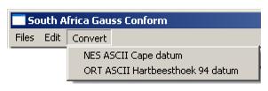
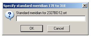
Note that the standard meridian for the Gauss Conform projection is available in the NES file header; however it is not available in the ORT file. The user will be prompted to enter the value.
If the converted binary files exist, then the index can be created directly from these files. Select the Files - File index menu item. Mutiselect the binary files and click the Open button to create the index.
BIL Geographic DEM Setup Procedure
The BIL geographic DEM is the generic base type for latitude - longitude spacial DEMs. Preconfigured versions of this base type are used for the following DEMs:
- SRTM (World)
- NED(NAD83)
- GTOPO30 (World)
- GridFloat (NAD83)
Select the Configure-Set System-GIS Setup Dialog from the menu and then select the Primary or Secondary DEM tab
In the Digital elevation model drop-down list, select the BIL geographic DEM. Note that the projection and datum do not change. This is the users responsibility.
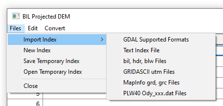
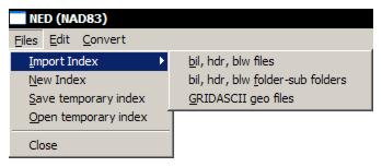
Click the File index button and then select the Files - Import Index menu item. The sub menu shown below, shows all available options for a BIL geographic DEM model. For each of these menu items, an open file dialog will appear. Select (or multiselect) the files and click the Open button.

GDAL Supported Formats
Currently GeoTIFF and IMG formats are supported.
Text Index File
bil, hdr, blw files
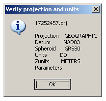
This is the ESRI format for both projected and geographic data. Three files are required to create the index. These must all be in the same directory. Open the bil file and the others will be automatically read. If the operation is successful, the projection data for this model will be displayed.
Read the details carefully. If this is not a geographic projection then the wrong BIL model was selected. Exit the file index and try the BIL projected model. The units will always be DD (decimal degrees). The Z units should be METERS; however, some USGS data in this format show NO (no units) in error.
SRTM hgt files
Mutiselect the hgt files to create the file index. Close the file index and set the datum to WGS84.
GRIDASCII geo files
These are ESRI GRIDASCII files which have been previously converted to a binary format. In the binary conversion a header is created with the extents and resolution of the file. The geo suffix means that this is a geographic file. There is no information on the datum in the file.
The Convert menu item on the BIL geographic main menu bar accesses the utility to convert the GRIDASCII ASCII file format to the Pathloss binary format. This step will also create the file index. Mutiselect the GRIDASCII files. A file save dialog will then open for the first file only in order to specify the directory for the binary files. All subsequent files will be saved in this directory.
MapInfo grd-grc files
Commercial DEM data is available in this file format. The file contains the datum and projection. If the file is not a geographic projection, then an error message will be returned to change the DEM model to BIL projected.
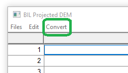
BIL Projected DEM Setup Procedure
Select the Configure-Set System-GIS Setup Dialog from the menu and then select the Primary or Secondary DEM tab
In the Digital elevation model drop-down list, select the BIL projected DEM. Note that the projection and datum do not change. This is the users responsibility.
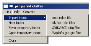
Click the File index button and then select the Files - Import Index menu item. The sub menu shown below, contains all available options for a BIL projected DEM model.
GDAL Supported Formats
Text index file
This is used for legacy Planet, Odyssey, and other RF design datasets. The DEM files consist of the following:
- Binary elevation data files
- Index file as shown below. The file consists of the file name, the edges in projected coordinates and the resolution:
height.bil 535590.0 545590.0 721330.0 731330.0 10.0 - Projection file - defines the datum and projection for the data. (In this example a zone 31 UTM projection using the WGS84 datum). Be sure to set the projection before clicking the File index button.
WGS-1984

	31

	UTM

	0.000000 3.000000 500000 0
Click the text index file menu and load the index file. The procedure uses the standard text import operation to define the file name, east, west, north and south edges and the cell size. Refer to the General program operation section for additional details on the use of this text import utility.
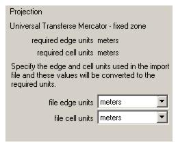
Note that the text import utility includes a Projection parameters button. This selection contains advanced DEM settings which are discussed at the end of this section and the required units for the edges and cell size. If the units in the data being imported are not the same as the required units, then set the edge and cell units in the two drop down lists. The data will be converted to the correct units.
bil, hdr, blw files
This is the ESRI format for both projected and geographic data. An open file dialog will appear. Open the bil file. If the operation is successful, the projection data for this model will be displayed.
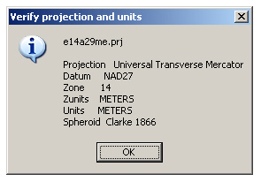
Read the details carefully. If this is not projected data, then the wrong BIL model was selected. Exit the file index and try the BIL geographic model. The units and the Zunits will always be meters. The user must set both the datum and projection as shown. In this example, a zone 14 UTM projection and NAD27 datum must be set.

GRIDASCII UTM Files
 These are ESRI GRIDASCII files which have been previously converted to a binary format. In the binary conversion a header is created with the extents and resolution of the file. The utm suffix means that the data is in a projected format (not necessarily a UTM projection). There is no information on either the datum or the projection in the file.The user must determine this information.
The Convert menu item accesses the utility to convert the GRIDASCII ASCII file format to the Pathloss binary format. This step will also create the file index. Mutiselect the GRIDASCII files. A file save dialog will then open for the first file only, in order to specify the directory for the binary files.
MapInfo grd-grc files
Commercial digital elevation data is available in this file format. The file contains the datum and projection. If the file does contain projected data, then an error message will be returned to change the DEM model to BIL geographic.
NED BIL INT16 Setup Procedure (LEGACY)
NED (National Elevation Dataset) is the primary elevation data product of the USGS. This is a seamless data set available nationally (except for Alaska) at resolutions of 1 arc-second (about 30 meters) and 1/3 arc-second (about 10 meters), and in limited areas at 1/9 arc-second (about 3 meters). In most of Alaska, only lower resolution source data is available. The elevations are for bare earth. The datum for all areas is NAD83.
USGS terrain elevation data is available for download in the following data formats:
- ArcGrid (proprietary ESRI format)
- GridFloat (4 byte IEEE floating point number)
- BIL_INT16 (2 byte integer format)
Only the BIL_INT16 and the GridFloat data formats are supported. The preferred format is BIL_INT16 due to the smaller data size, which results in a performance advantage. The setup procedure for the GridFloat data is given following this section.
The files are downloaded in a zipped format which includes a directory structure. Each directory contains several files including a header file (hdr), projection file (prj) and a world file (blw). These are required to create the NED file index. The elevation data is contained in the bil file.
- Select the Configure-GIS System-GIS Setup Dialog from the menu and then select the Primary DEM tab
- In the Digital elevation model drop-down list, select NED (NAD83). This DEM is a preconfigured type using the BIL geographic base type. The projection is automatically set to Geographic and the datum to the North American Datum of 1983. Set the specific region as required. Do not change these settings.
- The Setup button is used to set the directory when all files are in the same directory. NED files will be in different directories and this step is not required.
- Click the File index button and then select the Files - Import index menu item.
- To create an index for a single download directory, select the bil, hdr, blw files menu item. The BIL file selection dialog appears which includes a File directories selection. The default is always Use individual file directories. Go to the directory and select the bil file to create the index
- To create an index for multiple directories, select the bil, hdr, blw folder-sub folders menu item. Select the top level directory. The index will be created for this directory and all directories below this one. The directory structure should contain only NED elevation files.
- Close the File index and save the p5g file. This completes the setup procedure for the NED BIL_INT16 terrain database.
USA 3" Compressed Setup Procedure (LEGACY)
Three arc second terrain data for the United States in a compressed format is available for use with the Pathloss program. This data has been taken directly from the USGS 1:250,000 ASCII DEMs. The elevations in these files are in meters relative to mean sea level. The south-north resolution is 3 arc seconds. Below 50° the west-east resolution is 3 arc seconds. Between 50° and 70° the resolution is 6 arc seconds and 9 arc seconds above 70°.The error checking on these files consisted of the following verifications.
- Each elevation must be within the range specified for both the entire file and the specific column.
- The absolute value of all elevations, including the maximum and minimum values must be less than 10000 meters.
A total of 29 files did not pass this criteria and these were edited. The majority of errors involved the maximum elevation in the file. Other errors included extreme elevations (-32467) at the end of columns. These files have all been edited. None of the changes involved interpolating elevations. Most of the errors occurred at sea level.
All files are contained on a single CD-ROM and are organized in directories based on longitude under a main directory 3SEC_USA. The directory names are based on the longitude of the southwest corner of file e.g. W095. The file names are based on the longitude and latitude of the southwest corner. At latitudes less than 50º, the files have been split into two halves at the central longitude of the file. The letter L (left) or R (right) is appended to the file name. The file suffix is always cte (compressed terrain elevations). As an example, the file W095N44R.CTE represents the western half of the one degree block whose southwest corner is located at 44º north and 95º west. The file is located in the directory 3SEC_USA\W095 on the CD-ROM. The basic setup procedure is given below:
- Select the Configure-GIS System-GIS Setup Dialog from the menu and then select the Primary or Secondary DEM tab
- In the Digital elevation model drop-down list, select USA 3 sec compressed. The projection is automatically set to Geographic and the datum to the WGS84. Do not change these settings.
- Click the Setup button and set the main directory to the location of the 3SEC_USA directory.
- As this database uses a file naming convention in a fixed directory structure, the file index is not used and the setup procedure is complete.
USGS 7.5' Quad (USA) (LEGACY)
The USGS 7.5 minute terrain data has been superseded by the NED data.
The datum for this database is NAD27. All database operations will automatically transform NAD83 site coordinates to NAD27.
Each file contains elevation data for a 7.5 minute 1:24000 scale map quadrangle. The elevations have been determined by overlaying a square UTM grid onto the quadrangle. Both 30 meter and 10 meter resolutions were produced. Since the UTM grid system is not orthogonal to the latitude - longitude system that defines the map quadrangle, a skewing effect occurs. All columns do not contain the same number of elevation points and the first elevation in each column does not necessarily correspond to the same northing for all columns. For example, columns of data near the east or west edges of the quadrangle may be partially outside of the vertical boundaries as defined by lines of longitude. Therefore, only the points within the quadrangle boundaries are included in the file.
The USGS 7.5 minute files were supplied in ASCII format and are available directly through the USGS. These ASCII files must be converted to the Micropath 30m binary format as part of the setup procedure. The format and content of the ASCII files are described in National Mapping Program Technical Instructions, Data Users Guide 5, "Digital Elevation Models".
The following anomalies in the USGS 7.5 minute digital terrain data are handled:
- Elevations multiplied by a factor of 10
- 10 meter and 30 meters resolution data
- Various latitude and longitude offsets such as the 1.5 minute longitude offset for the island of Oahu and the 5 minute latitude and longitude offset for the Maui island group.
Select the Configure-GIS System-GIS Setup Dialog from the menu and then select the Primary or Secondary DEM tab
In the Digital elevation model drop-down list, select USGS 7.5 minute quad (USA). The projection is automatically set to UTM variable zone and the datum to NAD27. Do not change these settings.
Click the Setup button.
The 7.5 minute quad database can use a file naming convention or a file index. The file index is only intended for files that do not conform to the 7.5 minute quad format. All others must use the file naming convention.
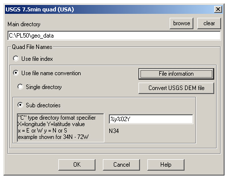
The two methods are described below.
File Index
If all files are in the same directory, click the Browse button and select the directory; however, it is often more expedient to assign the directories as part of the file indexing step.
Check the Use file index option and then click the OK button to close the Setup dialog. No further settings are required here for this method.
Click the File index button. The index can be created for existing 30m binary files. In this case, select the Files - File index menu item. Multiselect the 30m quad files and click the Open button to create the index.
If only the ASCII files exist, these must be converted to the binary 30m format. Select the Convert - USGS DEM menu item. Multiselect the ASCII dem files and click the Open button. A file save dialog will appear only for the first file for the sole purpose of specifying the directory to save the files in. Do not change the file name. All subsequent files will be saved in this directory. As part of the file conversion process the index will be created.
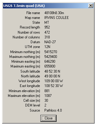
The File info menu item displays the header data of a converted 30m file.
File Naming Convention
The converted 30m files can be located in a single directory or a custom directory based on latitude and longitude. In both cases, the Main directory must be set. Click the Browse button and set this directory.
The program determines the required file based on the file names. The USGS file naming convention has the format "nnwwwNW" where:
- nn is the two digit northern latitude degree value, including leading zeros, of the southeast corner of the one degree block containing the quadrangle.
- www represents the three digit western longitude degree value, including leading zeros, of the southeast corner of the one degree block containing the quadrangle.
- N a single letter (A to H) designator defining the band of latitude north of the bottom (southern) edge of the one degree block.
- W a single number designator (1 to 8) defining the band of longitude west of the right (eastern) edge of the one degree block:
| Letter | Latitude | Number | Longitude |
| A | 0' to 7½’ | 1 | 0' to 7½ |
| B | 7½' to 15’ | 2 | 7½' to 15’ |
| C | 15' to 22½’ | 3 | 15' to 22½’ |
| D | 22½' to 30’ | 4 | 22½' to 30’ |
| E | 30' to 37½’ | 5 | 30' to 37½’ |
| F | 37½' to 45’ | 6 | 37½' to 45' |
| G | 45' to 52½' | 7 | 45' to 52½’ |
| H | 52½' to 60’ | 8 | 52½' to 60’ |
Select the Use file name convention option. Then select either Single directory or Sub directories. In the latter case, experiment with the format specifier for the directory name. This uses a C language printf notation. The directory structure must be created by the user.
Click the Convert USGS DEM file button. Multiselect the ASCII dem files and click the Open button. The files will be converted and saved in the specified directory structure.
To view the header information of a binary file, click the File Info button and then select the binary file name. The header shows the extents of the file in UTM coordinates and the horizontal datum.
Binary File Format
The USGS ASCII files must first be converted into a binary format. The file consists of a fixed record length for each column of elevation data; however, the record length may vary from file to file. The first record in each file is a header containing the following information:
| Table 4: Binary file header data |
| Bytes | Data type | Description |
| 1-2 | none | reserved |
| 3-4 | 2 byte integer | Record length |
| 5-6 | 2 byte integer | Number of columns |
| 7-8 | 2 byte integer | Number of rows |
| 9-12 | 4 byte integer | Minimum northing (meters) |
| 13-16 | 4 byte integer | Maximum northing (meters) |
| 17-20 | 4 byte integer | Minimum easting (meters) |
| 21-24 | ASCII | USGS map name |
| 25-64 | ASCII | Datum (NAD-27, NAD-83,) |
| 76 | ASCII | DEM level (1,2,3) |
| 77-78 | 2 byte integer | Minimum elevation (meters) |
| 79-80 | 2 byte integer | Maximum elevation (meters) |
| 81-120 | ASCII | Data Source |
| 121-122 | 2 byte integer | UTM zone (1-60) |
The remaining records in the file contain the elevation data - one record for each column. The columns run from west to east. The elevations in each column run from south to north. The first entry in each column is the easting (4 byte integer) of all elevations in the column. The next entry is the northing (4 byte integer) of the first elevation in the column. The remaining entries are the elevations in a 2 byte integer format. The northing of each successive column entry is obtained by adding 30 meters to the northing of the previous point. Since the binary file uses a fixed record length, some elevation points will be outside the boundaries of the map quadrangle. These elevations are set to the value -32000.
CDED (Canada) Setup Procedure (LEGACY)
CDED (Canadian Digital Elevation Data) files are available from www.geobase.ca in the USGS ASCII DEM file format. These are available in a 3 arc second and 0.75 arc second resolution corresponding to the 1:250 000 and 1:50 000 scale topographic maps, respectively. The higher resolution 0.75 arc second files are recommended and the following procedures apply to these files.
CDED file names
The download procedure for CDED files uses the Canadian National Topographic System (NTS) map naming convention. In the network display, the required CDED file names for a link can be found as follows:
- Select the Configure - Set GIS configuration menu item and verify that site coordinates projection is set to geographic.
- Select the Configure - Options - Network display options - Axis - Map grid menu item. Set the Map names to Canada 1:50,000 and the check the Show geographic grid and Show labels on grid options.
- Right click on a link and select the Map crossings menu item.
- A report will be created which show the required CDED file names for that link.
The files are downloaded in a zipped format. The 1:50,000 data is supplied in two files for the eastern and western sections.
ASCII to binary file conversion
The CDED ASCII files must first be converted to a binary format. This is a DTED type format with the suffix dtd. This step also populates the file index with the converted files and records the directory.
Select the Configure - Set GIS configuration and then select the Primary DEM tab
In the Digital elevation model drop-down list, select CDED (Canada). The projection is automatically set to Geographic and the datum to the North American Datum of 1983. Set the specific region as required. Do not change these settings.
Click the File index button and then select the Convert - USGS DEM menu item. A file open dialog will appear. Select the CDED ASCII files and click the Open button. This is a multi select file operation. A file save dialog will appear for the sole purpose of identifying the directory to save the converted files in. Do not change the file name. This directory will be used for all of the selected files. The files will be converted and the index will be created. The basic format of the binary files is given below:
- The elevations are 2 byte integers in the Motorola (big-endian) format.
- The elevations are organized in columns running from south to north starting in the south west corner. Each column begins with a header and ends with a check sum of the elevations.
- The elevations are defined at the intersection of the row - column grid lines. Note that in the BIL format, the data represents the average elevation in the cell at the center of the cell.
- The datum is NAD83.
- The spacial reference is geographic (latitude - longitude).
The CDED file index can contain both 1:50,000 and 1:250,000 files. In areas covered by files with both resolutions, the highest resolution file will be used.
CDED File Index
In the above step, the CDED file index was created as part of the ASCII to binary conversion. The index can also be created from the converted dtd binary files. In the CDED File index, select the Files - File index menu item. Multiselect the dtd files and click the Open button to create the index.
Data Verification
Each column of data includes a check sum of the elevations in that column. This procedure verifies the data integrity using this check sum. In the File index, select the Verify menu item. A Windows open file dialog appears. Multiselect the CDED files to be verified and click the Open button.
Pathloss 4 to Pathloss 6 DEM Cross Reference
The following table lists the Version 4 DEM selections and the corresponding Version 5 DEM. Note that some of the Version 4 DEMs have been discontinued.
| Table 5: Pathloss 4 to 6 DEM Cross reference |
| Version 4 DEM | Version 6 DEM | Datum |
| DTED-CDED indexed files - CDED | CDED Canada | NAD83 |
| DTED-CDED indexed files - DTED | DTED | WGS84 |
| DTED USDMA directory | DTED | WGS84 |
| DTED Canadian directory | DTED | WGS84 |
| DTED PL40 directory | DTED | WGS84 |
| CRC (Canada) | Discontinued | |
| GTopo30 Global 30 sec | GTopo30 World | WGS84 |
| Odyssey / Planet - UTM | BIL projected | UTM user specified zone and datum |
| Odyssey / Planet - Swiss grid | BIL projected | Swiss grid |
| Odyssey / Planet - UK Grid | BIL projected | UK Grid |
| Odyssey / Planet - Irish Grid | BIL projected | Irish grid |
| Odyssey / Planet - WGS84-MGI Austria | BIL projected | MGI Austria - coords in WGS84 |
| Odyssey / Planet- New Zealand Grid | BIL projected | New Zealand grid |
| Odyssey / Planet - Gauss Kruger | BIL projected | Transverse Mercator |
| USGS 7.5 Minute | USGS 7.5 minute quad | UTM variable zone NAD27 |
| Micropath 3 sec | Discontinued | |
| ESRI GRIDASCII GEO | BIL geographic | User specified datum |
| ESRI GRIDASCII UTM | BIL projected | UTM - user specified zone and datum |
| Phoenix 3 sec | Discontinued | |
| AUSLIG 3 sec | Discontinued | |
| South Africa NES | South Africa Gauss Conform | NES ASCII Cape datum |
| South Africa Gauss Conform | ORT ASCII Hartebeesthoek94 datum | |
| MDT Spain | Discontinued | |
| USA 3 sec compressed | USA 3 sec compressed | WGS84 |
| NED CONNUS | NED (NAD83) | NAD83 |
| NED Alaska | NED (NAD83) | NAD83 |
| SRTM | SRTM (World) | WGS84 |
| GRIDFLOAT - Connus | GridFloat (NAD83) | NAD83 |
| GRIDFLOAT - Alaska | GridFloat (NAD83) | NAD83 |
Clutter 1 and Clutter 2
The term clutter in the Pathloss program refers to land cover, terrain clutter, terrain morphology or in other words anything above the bare earth. Two separate clutter databases can be defined in the Clutter 1 and Clutter 2 tabs; however, unlike the terrain DEMS these do not function as a primary and secondary clutter. Only one clutter database can be active at any one time. The primary use of this arrangement is to calibrate clutter heights. There are three basic types of terrain clutter databases.
Clutter description only
The clutter database only contains a description of the clutter e.g. evergreen forest or developed high Intensity. There is no clutter height information. Unfortunately, this is the most common format and is the only type available from the USGS Seamless Server, The actual clutter database file simply contains an index to a clutter definition table. This table only provides the description and the color used to display the clutter. In the setup procedure, the user must edit the heights for each type of clutter to correspond to the area of interest.
Clutter heights only
The second type of database contains the actual clutter height above ground level. In this case, there is no description of the clutter available. This database does not use a clutter definition table.
Clutter heights determined as the difference between two DEMs
With some databases, clutter heights can be determined from the difference between the terrain elevation DEM and a second DEM defined in the clutter database.
An example of two DEMs which could be used in this context are NED and SRTM. NED by definition is bare earth. The SRTM elevations include buildings and tree cover to a certain extent by the nature of the data acquisition technique and this can be considered as a quasi composite elevation - clutter database. The difference between these two databases represent the clutter heights.
This technique can be used to calibrate the clutter heights in a description only clutter database. In the Terrain Data module, profiles can be generated using the description only database and the differential one. The results can be compared and the elevations in the clutter definition table edited accordingly.
This database does not use a clutter definition table.
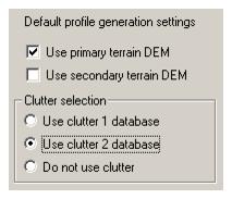
Choice of Clutter 1 and Clutter 2 tabs
One use of the description only clutter database is to provide a clutter backdrop in the network display using the colors in the clutter definition table. The description and heights are shown on the status bar for the cursor location. The database must be configured in the Clutter 1 tab for this functionality.
Clutter height databases should be defined in the Clutter 2 tab.
The use of clutter in terrain profiles is set under the Configure - Options - Program Options - Terrain Data - Profile generation menu item. This setting is common for all path profiles - point to point, point to multipoint, local and area study profiles.
Clutter Models
The following clutter models are available in the program:
- BIL projected clutter - base type
- BIL geographic clutter - base type
- NLCD 1992 (CONUS) description only - pre-configured BIL projected - Albers equal area conic - NAD83
- NLCD 1992 (Alaska) description only - pre-configured BIL projected - Albers equal area conic - NAD83
- GLCC (world) description only - pre-configured BIL geographic WGS84
- NLCD 2001 (CONUS) description only - pre-configured BIL projected - Albers equal area conic - NAD83
- NLCD 2001 (Alaska) description only - pre-configured BIL projected - Albers equal area conic - NAD83
- NLCD 2023 CONUS, Alaska and Hawaii - Included in the Automatic Terrain Management system
- NALC30 Canada, USA and Mexico - Included in the Automatic Terrain Management system
- CGLC100 Global - Included in the Automatic Terrain Management system
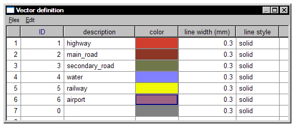
Clutter Definition Table
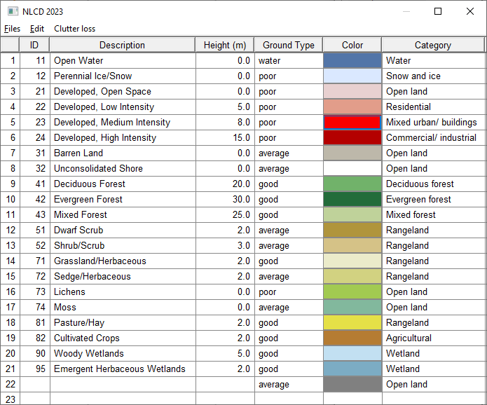
The clutter definition table is solely used for description only type clutter databases. The NLCD 2001 clutter definition table is shown here as an example. Note that this clutter database contains the ID, description and colors only. The height, ground type, and category columns are not part of this database. Details of these fields are given below.
Height
This is the height of the clutter above ground level in the current units setting (meters or feet). Note that in the preconfigured clutter databases, default heights have been entered. It is the users responsibility to set these heights to representative values for the specific area of the design. When a path profile is generated, a copy of the clutter definition table is saved in the pl5 file. This can be edited for the specific path independently of the main definition.
Ground Type
The ground types (poor, average, good, water) set the surface conductivity and the relative dielectric constant which are used to calculate the theoretical reflection coefficient. Differentiation between fresh water and salt water is based on the terrain elevation. If the elevation is zero and the ground type is specified as water, then the values for salt water are used: otherwise, the fresh water is assumed. In preconfigured clutter databases, the ground types have have been preset.
Clutter Category
In any link design, the clutter heights will determine the path clearance and these heights are sufficient. In local and area studies, additional data is assigned to clutter as follows:
- Location variability uses a log normal probability. The standard deviation is specified for each clutter category.
- Loss at the remote terminal / mobile due to local clutter. This loss will be a function of frequency.
There is no standard for clutter descriptions. In order to provide the additional definitions for local and area studies, the method proposed in the TIA document TSB-88.2-C is used here. Ten clutter categories are defined with the following descriptions:
- open land
- agricultural
- range land
- water
- forest land
- wetland
- residential
- mixed urban/ buildings
- commercial/ industrial
- snow and ice
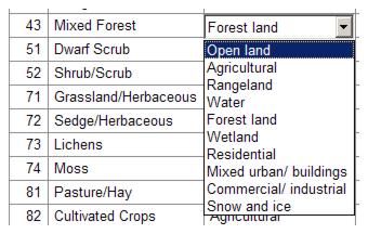
It is necessary to cross reference the clutter descriptions in the clutter definition table to these types. For each clutter description, double click on the Category column and select the appropriate cross reference.
Select the Clutter loss menu item. Select the clutter category from the drop down list. Default values for the clutter loss versus frequency are taken from TIA TSB-88.2-C. All values are user editable.
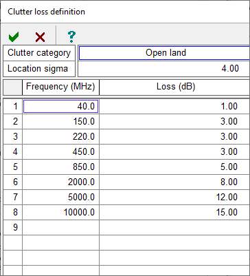
Note that this data is saved in the GIS configuration file (p6g). Local and area studies will use these values.
NLCD Setup Procedure (Legacy)
NLCD 1992 /2001 (National Land Cover Data 1992 /2001) is a 21-category land cover classification scheme. The NLCD classification is provided as raster data with a spatial resolution of 30 meters. This is a description only clutter database.
The setup procedure for NLCD 1992 and 2001 for CONUS and Alaska are essentially the same. The procedure given here is for NLDC 2001 (CONUS)
USGS land cover terrain elevation data is available for download in the following data formats:
- ArcGrid (proprietary ESRI format)
- GeoTiff
- BIL
- GridFloat
- IMG
Only the BIL format is supported. Download the required data files in this format from the USGS Seamless Data Distribution System. See the terrain data section at https://pathloss.com/pwiki for details. The files are downloaded in a zipped format which includes a directory structure. Each directory contains several files including a header file (hdr), projection file (prj) and a world file (blw). These are required to create the NLCD file index. The clutter ID data is contained in the bil file.
- Select the Configure - Set GIS configuration menu item and click the Clutter 1 tab. A description only clutter database must be setup in this tab to be available as a clutter backdrop.
- In the Clutter model drop-down list, select NLCD 2001 (CONUS). This clutter model is a preconfigured type using the BIL projected base type. The projection is automatically set to the Albers equal area conic for the USGS contiguous United States. The datum is set to the North American datum of 1983 with the CONUS region. Do not change these settings.
- The Setup button is used to set the bil file directory when all files will be in the same directory. The clutter files will be in different directories and this step is not required.
- Click the File index button and then select the Files - Import index menu item. The bil, hdr, blw files sub menu item will create an index for a single download directory using a file open dialog. Note the File Directories selection in this dialog. The default is always Use individual file directories. Go the directory and select the bil file to create the index
- The bil, hdr, blw folder-sub-folders sub menu will create index items for multiple directories. Select the top level directory. The index will be created for this directory and all directories below. The directory structure should contain only NLCD 2001 clutter files.
- Close the file index and click the Definition button. For each clutter description in the table, edit the associated clutter height. The initial values are default values and will not be applicable to your work area.
- Close the Clutter definition table and save the GIS (p5g) file. This completes the setup procedure for the NLCD 2001 clutter database.
Global Land Cover Characterization (GLCC - World) Setup Procedure (Legacy)
This is a “description only” clutter model and is the clutter companion to the GTOPO30 terrain elevation DEM. The model provides global coverage at a 30 arc second resolution using 17 clutter categories. The database consists of a single file - gigbp2_0ll.img (933,120,000 bytes). Details on downloading this file in a zipped format are in the Terrain Data section at https://pathloss.com/pwiki. The size of the zipped file gigbp2_0ll.img.gz is 27,460,036 bytes. Once the file has been downloaded, it must first be unzipped.
- Select the Configure - Set GIS configuration menu item and click the Clutter 1 tab. A description only clutter database must be setup in this tab to be available as a clutter backdrop.
- In the Clutter model drop-down list, select GLCC (World). This clutter model is a preconfigured type using the BIL geographic base type. The projection is automatically set to geographic and the datum to WGS84. Do not change these settings.
- Click the Setup button, then click the Browse button. Set the files of type to “all files” and navigate to the location of the gigbp2_0ll.img file. Click OK to complete the directory setting.
- Close the file index and click the Definition button. For each clutter description in the table, edit the associated clutter height. The initial values are default values and will not be applicable to your work area.
- Close the Clutter definition table and save the GIS (p5g) file. This completes the setup procedure for the GLCC (World) clutter database.
Clutter Heights Determined as the Difference Between Two DEMs Setup Procedure
In this setup procedure, clutter heights will be determined as the difference between SRTM and NED data. This choice determines certain aspects of the setup procedure; however the same concept will apply to any two DEMS, one of which is bare earth and the other a composite ground elevation and clutter.
Note that either the NED or SRTM could be configured as the primary DEM and the other as clutter. The choice is largely determined by the elevation backdrop. If one database contained embedded building data, then this would be set in the primary DEM to produce the elevation backdrop shown below. The bare earth database would be configured in the clutter tab.
For this example, assume that the primary DEM has been configured for the NED data. SRTM will be used in the clutter tab. See the SRTM setup procedure above for details on SRTM file names and the download procedure.
- Click Configure - Set GIS configuration and select the Clutter 2 tab.(Leave the Clutter 1 tab free for a “description only” model to allow clutter backdrop generation.
- Only the BIL geographic and BIL projected clutter models can be used in a difference between two DEMS configuration. As SRTM is geographic, select the BIL geographic clutter from the Clutter model drop down list.
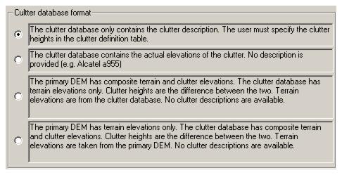
- Click the Setup button and select the fourth clutter database format - “The primary DEM has terrain elevations only. The clutter database has composite terrain and clutter elevations...”
- If all SRTM files will be located in the same directory click the Browse button and set this directory; otherwise, click the Clear button to erase directory edit box. The directory for each SRTM files will be set when the file index is created. Click OK to close the Setup.
- Click the File index button and then select the Files - Import index menu item. Select the SRTM hgt files menu item. Multiselect the SRTM files to create the index.
- Close the File index and save the GIS (p5g) file. This completes the setup procedure for the two DEM differential clutter.
Combining Clutter Height and Clutter Type (Legacy)
See also Combining Clutter Height and Clutter Type
The following is a method for manually configuring description clutter using height based clutter
Create a link in the Network display and left click on the link. Select the Terrain data menu item.
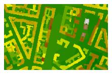
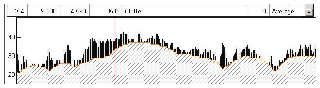
Select Operations - Generate profile and set the options as shown above. The BIL geographic clutter has been setup for the SRTM data. Click the green check to generate the profile. The resulting profile below shows the clutter as vertical lines. The heights are shown in the table using the description “Clutter”.
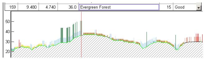
Now repeat the profile generation using the NLCD 2001 clutter model. The resulting profile below shows the clutter as colored lines on the profile with the full description in the table. Remember that the clutter heights in this case are the users values and these will be edited based on the SRTM profile. For buildings, the SRTM clutter heights are realistic, For tree cover, there will be some correction as the radar signal would penetrate to some degree depending on the density. For point to point link feasibility studies, a conservative estimate would be assume that the SRTM tree heights are 50% of the actual values.
The corrections can be made for the specific profile by double clicking on any line in the Structure column or globally set in the GIS configuration.
BIL Projected and BIL Geographic Clutter Models (Legacy)
The previous example of clutter derived from two DEMs used the BIL geographic clutter model to configure SRTM data in the Clutter 2 tab. The predefined clutter models use the following generic BIL types.
- NLCD (CONUS) - BIL projected NAD83 datum, Albers equal area conic - USGS contiguous United States
- NLCD (Alaska) - BIL projected NAD83 datum, Albers equal area conic - USGS Alaska
- GLCC (World) - BIL geographic WGS84 datum.
A definition table has been created for each of these predefined models.
These models can be configured for other clutter data sources. The user must set the datum and projection for the specific data. The following are general guidelines when configuring a clutter model with the BIL projected or geographic base types.
Click the Setup button and select the clutter database format. This selection is only available in the BIL geographic and projected clutter models.
BIL Geographic Clutter Setup Procedure
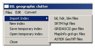
Select the BIL geographic clutter model from the Clutter model drop-down list and then click the File index button. Select the Files - Import index menu item. The sub menu shown below, contains all available options for a BIL geographic clutter model.
bil, hdr, blw files
This is the ESRI format for both projected and geographic data. Open the BIL file. If the operation is successful, the projection data for this model will be displayed.
Read the details carefully. If this is not a geographic projection then the wrong BIL model was selected. Exit the File index and try the BIL projected model. The units will always be DD (decimal degrees). If the Z units are NO (no units), then this clutter model is a “description only” type and a definition table must be created. The user must set the datum as shown The projection will always be geographic (latitude - longitude).
The actual interpretation of the data (an index to a descriptor table, the actual clutter elevations, composite ground and clutter elevations or ground elevations only) is left to the user. Note that this selection would be used to configure a NED DEM for clutter derived from two DEMs with SRTM in the primary DEM tab and NED in the Clutter 2 tab.
SRTM hgt files
This option has been described in the above setup procedure for clutter derived from two DEMS using the fourth option in the clutter database format. Mutiselect the hgt files to create the file index. Close the File index and set the datum to WGS84.
GRIDASCII geo files
These are ESRI GRIDASCII files which have been previously converted to a binary format. In the binary conversion a header is created with the extents and resolution of the file. The geo suffix means that this is a geographic file. There is no information on the datum in the file. The actual interpretation of the data (an index to a descriptor table, the actual clutter elevations, composite ground and clutter elevations or ground elevations only) is left to the user.
The Convert menu item on the BIL geographic main menu bar accesses the utility to convert the GRIDASCII ASCII files to the Pathloss binary format. This step will also create the file index. Mutiselect the GRIDASCII files. A file save dialog will then open for the user to specify the directory to save the binary files in.
MapInfo grd-grc files
Commercial clutter data is available in this file format. The file contains the datum and projection. If the file is not a geographic projection, then an error message will be returned to change the clutter model to BIL projected.
If the file is a “description only” clutter model, then a clutter definition file will be automatically created. In general, there is no clutter height information and the user must add these heights and edit the ground types and the clutter category cross reference.
ASTER Geo Tiff files
This option would only be used for clutter derived from two DEMS using the fourth option in the clutter database formats. Mutiselect the tif files to create the file index. Close the file index and set the datum to WGS84.
BIL Projected Clutter Setup Procedure
Select the BIL projected clutter model from the Clutter model drop-down list and then click the File index button. Select the Files-Import index menu item. The sub menu shown below contains all available options for a BIL projected clutter model.
Text Index File
This is used for clutter data from legacy Planet, Odyssey, and other RF design programs. These are “description only” clutter databases consisting of the following files:
Binary Clutter Data Files
Index file - This file consists of the file name, the edges in projected coordinates and the resolution.
clut1 499975 600025 199975 300025 50

clut2 599975 700025 199975 300025 50

clut3 699975 800025 199975 300025 50
Menu file - This file lists the id numbers in the binary clutter data file and the corresponding description.
148 foret

222 foret_degradee_plantation

130 zone_urbanisee

105 zone_industrielle

84 village

248 sol_nu

70 eau

191 marecage
Projection file - Defines the datum and projection for the data - in this example, a zone 32 UTM projection using the WGS84 datum. Be sure to set the projection before clicking the File index button.
WGS-84

32

UTM

0 9 500000 0
Click the Text index file menu and load the index file. The procedure uses the standard text import operation to define the file name, east, west, north and south edges and the cell size. Refer to the General program operation section for additional details on the use of this text import utility.
Note that the text import utility includes a Projection parameters button. This selection contains advanced DEM settings which are discussed at the end of this section and the required units for the edges and cell size. If the units in the data being imported are not the same as the required units, then set the edge and cell units in the two drop down lists. The data will be converted to the correct units.

bil, hdr, blw files
This is the ESRI format for both projected and geographic data. Open the BIL file in the dialog. If the operation is successful, the projection data for this model will be displayed.
Read the details carefully. If this is not projected data, then the wrong BIL model was selected. Exit the file index and try the BIL geographic model. The units will always be meters. If the Zunits are NO (no units), then this clutter model is a “description only” type and a definition table must be created. The user must set both the datum and projection as shown. In this example, a zone 14 UTM projection and NAD27 datum must be set.
The actual interpretation of the data (an index to a descriptor table, the actual clutter elevations, composite ground and clutter elevations or ground elevations only) is left to the user.
GRIDASCII utm files
These are ESRI GRIDASCII files which have been previously converted to a binary format. In the binary conversion a header is created with the extents and resolution of the file. The utm suffix means that the data is in a projected format (not necessarily a UTM projection). There is no information on either the datum or the projection in the file.The user must determine this information. The actual interpretation of the data (an index to a descriptor table, the actual clutter elevations, composite ground and clutter elevations or ground elevations only) is left to the user.
The Convert menu item on the BIL projection main menu bar accesses the utility to convert the GRIDASCII ASCII file format to the Pathloss binary format. This step will also create the file index. Mutiselect the GRIDASCII files in the file open dialog. A file save dialog will then open for the user to specify the directory to save the binary files in.
MapInfo grd-grc files
Commercial clutter data is available in this file format. The file contains the datum and projection. If the file is a geographic projection, then an error message will be returned to change the clutter model to BIL geographic.
If the file is a “description only” clutter model, then a clutter definition file will be automatically created. In general, there is no clutter height information and the user must edit the heights, ground types and clutter category cross reference.
Data Parameters in BIL Projected and Geographic Files
In the pre-configured clutter models, NLCD and GLCC, the data parameters are correctly set. In the case of the base BIL geographic and projected clutter models, some parameters may require changes.
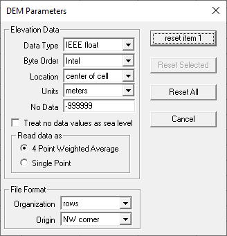
Data type
Most description only clutter databases typically use an 8 bit integer.
Byte order
The byte order is only a consideration when the data type is larger than an 8 bit integer. An incorrect setting will result in no data or very erratic data.
Location
This must be set to the “center of cell” for BIL data files.
Units
Units are not applicable to “description only” clutter models.
No data value
This is not used in “description only” clutter databases. In this case the no data value is specified in the clutter definition table.
Treat no data values as sea level
This option is not applicable to “description only clutter models and should not be checked.
Read data as 4 point average or single point
On “description only” clutter models, this must be set to a single point read. The 4 point weighted average can be used for clutter derived from two DEMs and clutter models containing clutter elevations.
File format organization
This must be set to rows in a BIL file.
File format origin
The file data origin can be in the NW corner or the SW corner. If the clutter backdrop display is upside down, change the origin to the opposite setting.
Backdrop Imagery
Raster images in the usual graphic formats (TIFF, GeoTIFF, BMP, JPEG and PNG) can be used as a backdrop in the network display. The only requirement is that the image must have a geographic reference so that the sites can be correctly shown on this backdrop. This can be accomplished by the following two methods:
- The image has been produced with a rectangular projection (e.g. UTM zone 32 - ED50 datum). The projection grid is aligned horizontally and vertically with the image edges. In this case there can be multiple images on the network display if they all use the same rectangular projection. This method is referred to as edge referenced. The projected coordinates of the west, east, south and north edges of the image serve as the geo-referencing information.
- All other images must be manually geo-referenced. The user must provide the coordinates (either latitude and longitude or projected coordinates) for several points on the image. Only a single image can be displayed in this case. An affine transformation is used to position the sites and vector data on the image.
Note that when backdrop imagery is present, the projection used by the network display must be the same as the image. If a manually geo-referenced image is used in a small area of the overall network, then severe distortion can occur outside this area.
Click the Backdrop tab. If the datum and projection of the image are known, then set these now and then click the Setup button.
If the image files will all be located in the same directory, click the Browse button and set the Main directory.
Select the required geo-referencing method.
Edge Referenced File Index
Click the File index button. The required data entries are: file name, west, east, south and north edges and the file type. The cell size (image resolution) will be calculated and is for information purposes only. The Show check box is used to hide the selected image. Select the Files - Import Index menu item. The following methods are available to import a file index entry:
Text file index
The image files are supplied with an index file and a projection file as shown in the examples below for legacy Planet type data:
lagos.tif 535590.0 545590.0 721330.0 731330.0 10.0

Projection file

WGS-1984

31

UTM

0.000000 3.000000 500000 0
The index is imported into the File index using the standard text file import utility described in the General program operation. Select the Text file index menu item, load the index file and carry out the import procedure.
Set the backdrop datum and projection as defined in the projection file.
GeoTIFF file
GeoTIFF files contain both the image and the geo-referencing information. Select the GeoTIFF file menu item and load the file. The GeoTIFF parameters will be displayed. The exclamation icon indicates that sufficient information is available to geo-reference the image. Click the Create index button to complete the index. The datum and projection will be automatically set.
MapInfo tab file
A MapInfo tab file also contains geo-referencing information for an image file. Select the MapInfo tab file menu item and load the file. A MapInfo tab file is used for various purposes and several errors can occur:
- The file is not a raster image.
- The file cannot be edge referenced.
In the latter case, reload the MapInfo tab file in the Manual geo-referencing section
Create 8Bit Palette Bitmap
Very large 24-bit color ortho imagery files (~350 Mbs) are available from the USGS. The processing time for a single file generally results in poor performance. If the network display includes several of these files, the memory mapping will fail. The solution is to convert the file to an 8 bit palette version. This reduces the file site by a factor of 3 for 24 bit color and 4 for 32 bit color. Place the cursor on the line to convert and select the Create 8 bit palette bit map menu item.There is no perceptible change in the image quality. Note that this process can take considerable time to complete. There is no progress status indicator at this time.
In some cases the file may fail to load due to memory limitations. An external utility cnvt24_8.exe is provided to create the 8 bit palette bit map outside the Pathloss program. Note that the resultant file is a bitmap. If the source file was a GeoTIFF file, then the geo-referencing information in that file cannot be transferred to the bitmap. A good way to start is to create the index with the GeoTIFF file. Attempt to convert the file to an 8 bit palette bit map using the function in the File index. If this succeeds, the index will be modified for the new bitmap file name and the file type will be set to bmp. If this fails, then use the external cnvt24-8 program. Then manually change the file name and file type in the File index.
Create bitmap array
Situations may occur where performance can be improved by breaking up a large image into smaller bitmap images and then using a subset of these images for the network display. This feature is only available using edge referenced backdrops.
In the File index, select the Files - Create bitmap array menu item. Set the number of rows and columns as required and click OK. The bitmaps and the associated new index items will be created. The existing image index will not be erased, but its “show” status will be turned off.
Manual Geo-Referencing
Click on the Geo-reference button to open the geo-reference window. Note that the button name and function changes depending on the geo-reference method selected in the Setup section.
Procedure
Select the File - Image file and load the required image file. Note that the zoom and pan features (including the mouse wheel zoom) are the same as used in the network display.
Note that if the image is a GeoTiff file, then the geo-referencing information in the files is transferred to the display. Click the Finish button to complete the operation.
The basic procedure is to identify a pixel on the display and enter the coordinates for that pixel. These coordinates must correspond to the backdrop imagery projection. In order to select a pixel, the cursor must be in the selection mode. Click the selection cursor on the tool bar.
Pixel Selection
Move the cursor to a point with known coordinates and click the left mouse button. The location is identified with a red square. Typically, this would be the intersection of grid lines or some landmark with known coordinates. The values for the X and Y pixel location will be entered. Enter the coordinates of this point in the edit boxes labelled Projected X and Y. An optional label for the point can also be entered. Click the Add point button to add this geo-referenced point. The point will now be marked with a blue square.
Editing a Geo-referenced point
Select a point by clicking on its Label name in the first column of the geo-point list. This fills in the edit boxes with that point’s information. To edit the data, make the required changes in the edit boxes and click the Modify point button to update the data. To delete the point, click the Delete point button.
Usage Hints
At least 3 points are required to fully geo-reference an image. Adding more points can greatly improve the accuracy for certain projections. For UTM and similar projections, three points are sufficient, whereas geographic (latitude - longitude) coordinates may require more points for the desired accuracy. For best results, the points should be spaced out around the entire image with a good sampling of the variations in both the x and y axis. Points in a line are not suitable for geo-referencing and a warning may be generated. Once 3 points have been entered, the dialog bar will report the calculated coordinates to the right of the geo-point list. You can use this to check the accuracy of the calculation.
Problem geo-referenced points may be recognized by checking the error columns in the geo-point list. If any points have an error that is abnormally large compared to the other points, there may be a problem with its coordinates.
When the geo-referencing is complete, click the Finish button. The message shown below will appear if the edges of the file can be used to geo-reference the image. This edge referenced method is recommended due to a simpler calculation and the ability to tile images.
MapInfo tab file
MapInfo tab files contain the geo-referencing information. Select the File - MapInfo tab file menu item and open the required tab file. The image file will be loaded and displayed and the geo-referenced data will also be displayed. Click the Finish button to finalize the operation.
Vector Data
Click the Vector Data tab in the Configure Geographic System dialog. GeoJSON, ESRI Shapefiles, MapInfo mapfiles and the legacy Planet vector data text files are supported. The procedure for each of these is given below.
GeoJSON
GeoJSON is a format for encoding a variety of geographic data structures. https://geojson.org/
There are two methods for using GeoJSON data in Pathloss 6. As individual files and as a directory of files.
Individual Files
- Click the File Index button.
- Click Files Import - Vector Files.
- Select the GeoJSON files that you would like to import and click Open.
Vector Tile Folder
- Click the File Index button.
- Click Files Import - Vector Tile Folder.
- Select the folder that contains the desired GeoJSON files.
- Pathloss will index the folder and show it as one entry in the index. This allows a cleaner index and allows adding files with out re-indexing.
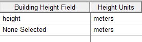 For both methods the user must select the height field by double clicking the Building Height Field and selecting the appropriate data field. Once the height filed is set the user must select the height units by double clicking the Height Units field and selecting the appropriate units from the drop-down list.
Pathloss will attempt to set the projection and datum information automatically. If the program fails to do this, the projection information will be displayed so the user can set it manually in the Vector Data tab of the Configure Geographic System dialog.
ESRI Shapefiles
It is the users responsibility to determine and set the associated projection and datum.
Click the File index button and then select the Files - ESRI shapefiles menu item. Load the shapefile and the index will be created.
This completes the setup procedure for the ESRI shapefile. Only the vector outlines will be drawn, There is no provision to set the vector line attributes.
MapInfo Mapfile
MapInfo Mapfiles include the datum and projection.
Click the File index button and then select the Files - MapInfo Mapfile menu item. Load the corresponding MapInfo Tab file and the index will be created. The datum and projection will be automatically set.
This completes the setup procedure for the MapInfo Map files. Only the vector outlines will be drawn, There is no provision to set the vector line attributes.
Building Vector Files
Building vector data which includes building heights is available in both the GeoJSON, ESRI Shapefile and the MapInfo mapfile format. Please see Terrain Data Sources for sources of building vector data.
Terrain profiles with building heights can be created from these files. Note the column labelled Building Height Field in the Vector File Index. When the index is first created, this will be set to “None Selected”. Double click on this cell and a drop-down list will appear with all of the available fields. Select the field that corresponds to the building heights.
In the Network display, the vector data will be shown as normal. When a profile is generated, the program will check if the Building height field has been set (correctly or incorrectly), Clutter 1 and Clutter 2 will be disabled and the program will attempt to read the building height from the vector file.
Planet Type Vector Data Files
The following files are used in this vector format:
Index file - This gives the individual vector file name, the extents and a description of the specific vector.
highway 540421.0 544619.0 721331.0 731331.0 highway

main_road 535595.0 545595.0 721331.0 731331.0 main_road

secondary_road 535595.0 544911.0 721331.0 731331.0 secondary_road

water 535595.0 545595.0 721331.0 731331.0 water

railway 536188.0 540331.0 721331.0 731331.0 railway

airport 535595.0 537475.0 725453.0 729981.0 airport
Projection file - This file is used to set the projection and datum in the Vector Data tab
GRS-1980

31

UTM

0.000000 3.000000 500000 0
Menu file - This file contains the index and description of each vector type. This is used to create a vector definition to set the colors and line styles for each vector.
1 highway

2 main_road

3 secondary_road

4 water

5 railway

6 airport
Set the datum and projection for the vectors.
Click the Setup button. Click the Browse button and set the vector files directory.
Click the File index button. Then select the Files - Import text file index menu item and load the index file. The standard text import utility is used to import the index. Refer to the General program operation section for details.
Click the Edge - cell units button. This shows the required units for the currently defined projection. If the units in the import data are not the same as the required units, then set the edge and cell units in the two drop down lists. The data will be converted to the correct units.
Click the Definition button to set the vector colors, line style and line widths. Select the Files - Import text file index menu item and import the menu file for the vectors. The standard text import utility is used to import the menu. Only the ID and description is available in the menu file. The line colors, width and style are set by the user.